1.2. Scientific context

1.2.1. Ice

1.2.1.1. Ice crystallographic structure

    Ice is composed of water molecules (H2O) which form a hexagonal crystallographic structure in pressure and temperature conditions met on Earth. This hexagonal configuration of molecules linked by hydrogen bonds leads to the hexagonal symmetry, observable on snowflakes. This hexagonal plane is called the basal plane and can be defined in space by a normal vector of this plane called \(c\)-axis. If all basal planes of molecules have the same orientation, it forms a single crystal of ice, represented in Figure 1.1. Such crystal can contain some failures like molecule missing or atom switch [Chauve, 2017].

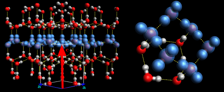
Fig. 1.1 Crystallographic strucure of ice. Blue molecules are from the same basal plane. Picture from [Chauve, 2017]

1.2.1.2. Plastic deformation mechanisms

Sometime can appear dislocations that are linear failures forming a discontinuity of the crystal lattice, meaning a non full plan of molecules missing, forming a tension and a compression zone in the crystal represented on Figure 1.2. A dislocation is spreading accomodating deformation by gliding through the crystal. Dislocations gliding are the main mechanism for plastic deformation in ice.

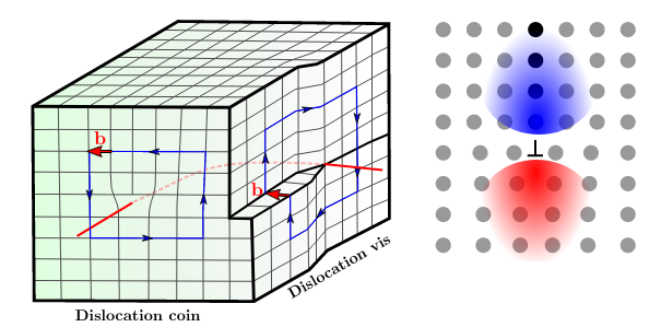
Fig. 1.2 (Left) Shematic representation of dislocation with dislocation lines and in red . (Right) Plane view of a dislocation with compression zone (blue) and tension zone (red). Pictures from [Chauve, 2017]

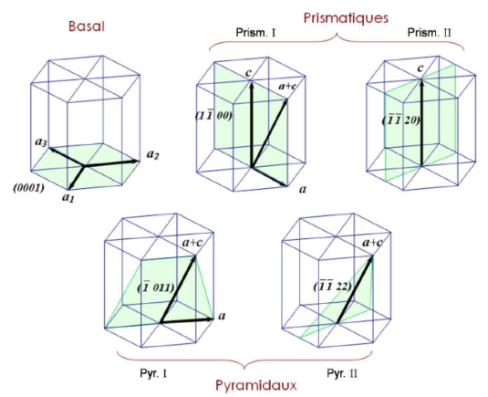
Fig. 1.3 Dislocations theorical slip planes for ice. Picture from [Chauve, 2017]

1.2.1.3. Ice polycrystal

    Ice in natural conditions is mostly observed as a polycrystal material, formed by several grains (single crystals) with different crystallographic orientations size and form like on Figure 1.4. A grain boundary is a boundary between two crystallographic orientations, which can have a role to create or delete dislocations. There are several types of grain boundary referring to the rotation angle defined between the orientations of the two grains. Ice creep has been widely studied for a long time, and in particular the interplay between microstructure evolution during creep and mechanical response, at various temperature and stress conditions [Jacka and Maccagnan, 1984]. The dynamic recrystallisation has a role impacting the rate of deformation, the microstructure and the crystallographic orientations in the polycrystal (textures). Many open questions remains related to this mechanism of recrystallization.

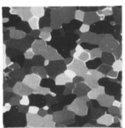
Fig. 1.4 Microstructure observed at \(2779 m\) deep in Vostok drilling. Picture from [Thorsteinsson et al., 1997]

1.2.2. Recrystallisation

    As said before, plastic deformation of crystalline material is due to dislocation propagation when submitted to a stress field. The accumulated strain results in an increase of the density of dislocations. In order to reduce the energy stored by the dislocations produced, recrystallisation mechanisms will be activated and will lead to a modification of the crystal network. There are two types of recrystallisation :

• Static recrystallisation which happens after the deformation during annealing for metal materials.

• Dynamic recrystallisation which happens during the deformation. We will focus on this process.

    Recrystallisation consequence is to transform the crystalline network to have a less stored energy within the microstructure. There are 3 main mechanisms that rule recrystallisation :

• Grain boundary migration : Dislocations tend to accumulate next to grains boundaries. When density is too high, grain boundary might move through dislocations and absorb them. This mechanism leads to a modification of grain boundary’s form, creating sawtooth boundaries.

• Grain sub-boundary formation : When dislocations arrange into an alignment, it can create a sub-boundary, not enough misoriented to be classified as a true boundary. If misorientation increase, it can evolve into a grain boundary leading to the creation of a new grain.

• Nucleation : “Nucleation” is the formation of new grains at grain boundaries or triple junctions, as a response of a too high concentration of dislocations. The nucleation can be the result of a local grain boundary migration also known as bulging [Chauve et al., 2017] or it can result from more complex mechanisms that are still quite poorly known.

The Figure 1.5 shows these recrystallisation mechanisms on a strained polycrystal with a schematic way.

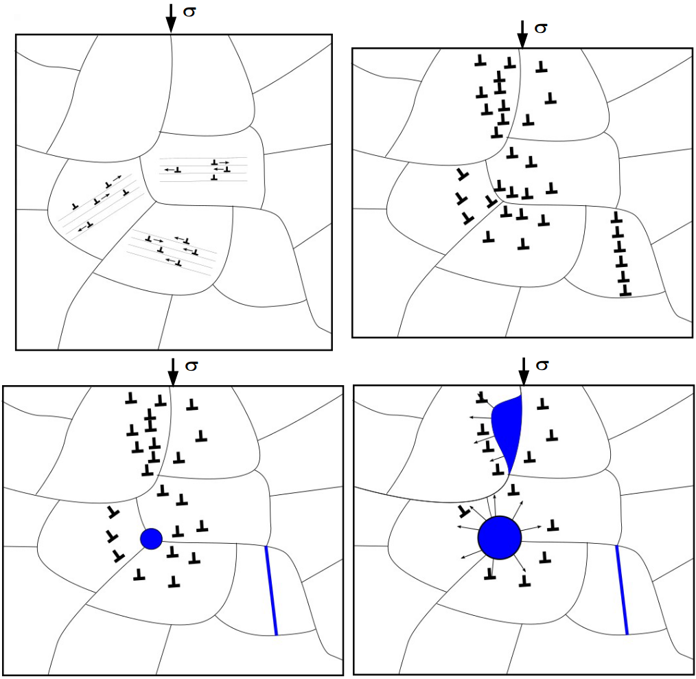
Fig. 1.5 Recrystallisation mechanisms : dislocation accumulation next to grain boundary, sub-boundary formation, boundary migration and nucleation . Picture from Thomas Chauve

    Nucleation mechanisms are not well predictible because of the difficulty to identify which mechanisms it is. In addition, observe by experiment these mechanisms is not an easy task. Indeed, “nucleus” appears with a size much smaller than the limits of the actual observation capabilities. That why model experiences are made with aim to indentify nucleus and their formation process. In the study, we focused on studying the localization of new grains.

1.2.3. Experimental tools

1.2.3.1. Uniaxial Compression

    To obtain data for studying ice deformation behaviour, the mostly done experiment in literature is uniaxial compression because in natural conditions, ice is deformed by the accumulation of ice layers. It gives a vertical compression that can be simulated in cold room. A parallelipedic ice sample is submitted to compression under a constant applied load or stress. The results of the experiments used in this study have been made by Thomas [Chauve, 2017]. As we can see in Figure 1.6, representing a schematic view of the experiment where \(\sigma\) correspond to the compression applied, the microstructure of columnar ice is easier to observe because of the large grain and the possibility to apply a distructive AITA analysis (see next). This type of sample can be produced in the laboratory. The samples used here have a size of \(90\times 90 \times 15 mm^3\).

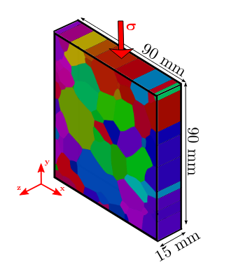
Fig. 1.6 Colomnar ice sample used in experimentions with \(\sigma\) the applyed strain. Picture from [Chauve, 2017]

1.2.3.2. Orientaions maps

    To determine the orientations of ice crystals, the method used is an optical measurement of a thin section of ice. The goal is to calculate the orientation of the \(c\)-axis of basal plane. To do that, it is a succession of measurements of light intensity, turning the thin section between 2 cross polarizer. This result in an intensity curve in function of the angle of rotation of the thin section. This curve is characteristic of \(c\)-axis and the polar coordinates \(\Phi\) and \(\Theta\) can be calculated by an appropriated regression see Figure 1.7 (right). This is done by mean of the Automatic Ice Texture Analyzer (AITA) of D. Russel-Head and C. Wilson [WILSON et al., 2007] that provides \(c\)-axis orientations measurements with a resolution of about 3° on thin sections as large as \(12\times 12 cm^2\), with a spatial resolution as low as \(5\) microns. In the presented experiments, the used resolution is of \(20\) microns. Orientation map of \(c\)-axes can be measured that give results like we can observe on Figure 1.7 (left). A Python package, named xarrayaita, has been developed by Thomas Chauve to manipulate the results of AITA using xarray.

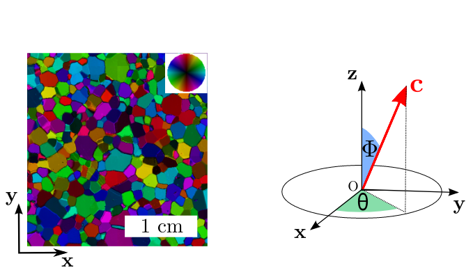
Fig. 1.7 (Left) Map of orientations obtain by AITA with colorscale corresponding to the stereographic projection of \(c\)-axis in plane \(xOy\). (Right) Definition of \(\Phi\) and \(\Theta\) angles defining \(c\)-axis measured by AITA. Picture from [Chauve, 2017]

1.2.3.3. Simulation fields

    In order to evaluate strain and stress fields for a given microstructure, a full field model has been used to make estimations. The model CraFT has been developed by [Moulinec and Suquet, 1998] and used with the elastoviscoplastic constitutive equation adapted to ice material proposed by [Suquet et al., 2012]. Details of this equation have been explained by Thomas [Chauve, 2017]. This model allows us to calculate equivalent strain and stress fields prior to recrystallization. They were calculated using python package xarraycraft.

1.2.4. Machine learning tools

1.2.4.1. Machine learning algorithms

    Machine learning methods allows user to extract informations from data which could be too much hidden in mass. From dimension reduction to regression or classification, many kind of algorithms have been developed and upgraded over time. Methods can be dissociated in 2 categories :

1.2.4.1.1. Unsupervised learning

Unsupervised learning methods aim is to let the algorithm determine paterns and correlations that we didn’t know before start learning. There is no variable to predict in the data. The program “explore” data to find some correlations which can characterize data overall. Popular exemples of unsupervised leaning method are clustering methods. Indeed, the goal of these methods, like k-means, hierarchical clustering or gaussian mixture models, is to determine categories of individuals into data from the variable values (Figure 1.8). Data trues classes are not used for the learning, involving that algorithms evaluate individuals in relation to a discrimination criterion only using variables distribution. If the number of true classes is unkown, clustering algorithms allow to estimate the number of classes. Otherwise, when the true number of classes is known, clustering methods can be used as classification method. Next, we used k-means method as a binary classification method (see K-means).

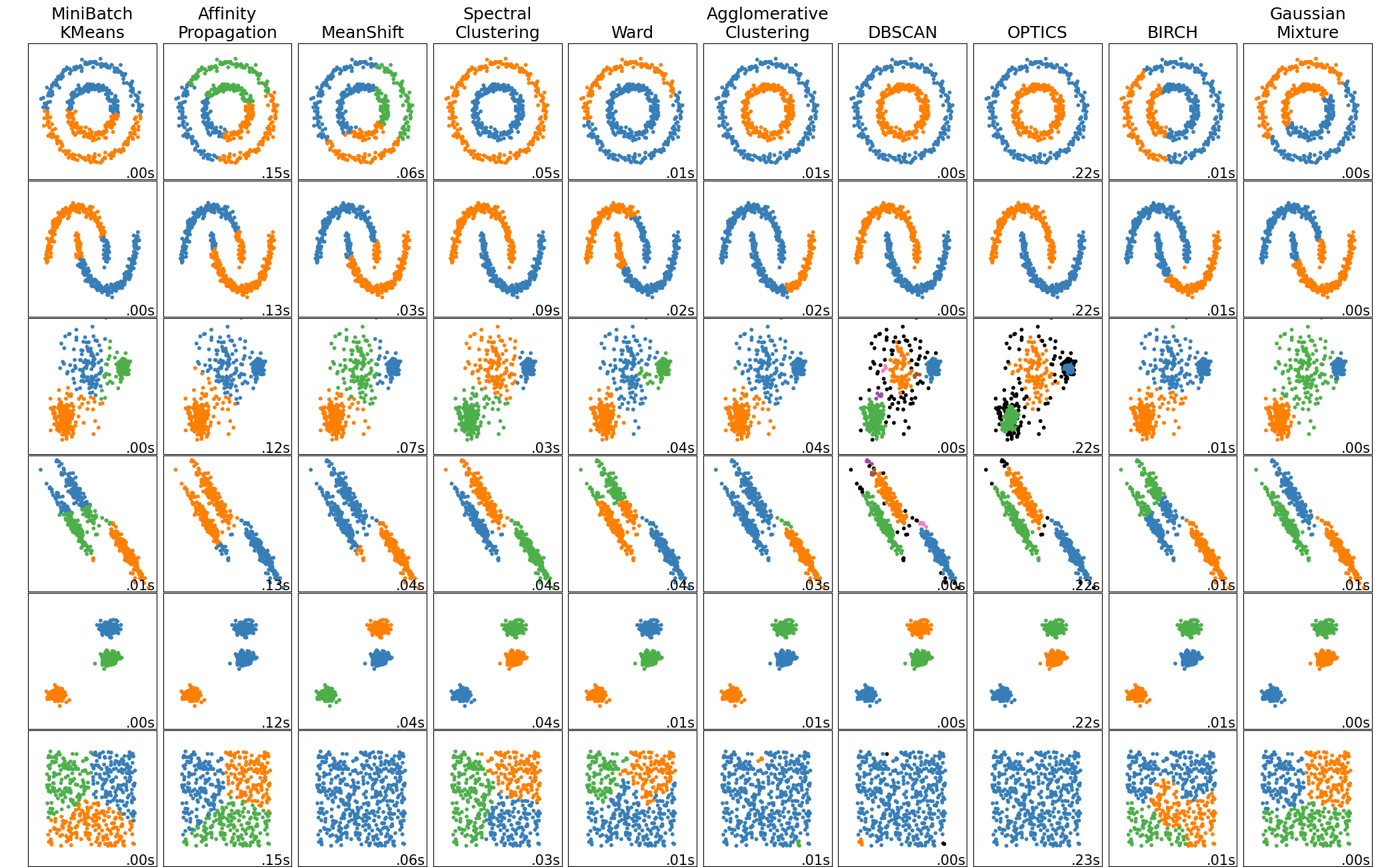
Fig. 1.8 Comparison of clustering algorithms in scikit-learn. Picture from Scikit-learn documentation

Another kind of frequently used unsupervised methods are dimensional reduction algorithms. When the number of data variable is too high to be undertood overall, it is possible to apply tranformation on data to down dimension, using methods like PCA or t-SNE, and make a projection of data into a lower dimensional space (Figure 1.9). In our case, we used these two methods in the data exploration process (see Data exploration). The tranformations applied on data are specific to algorithm but always try to keep distance between individuals and be representative of the distribution of individuals in the true space.

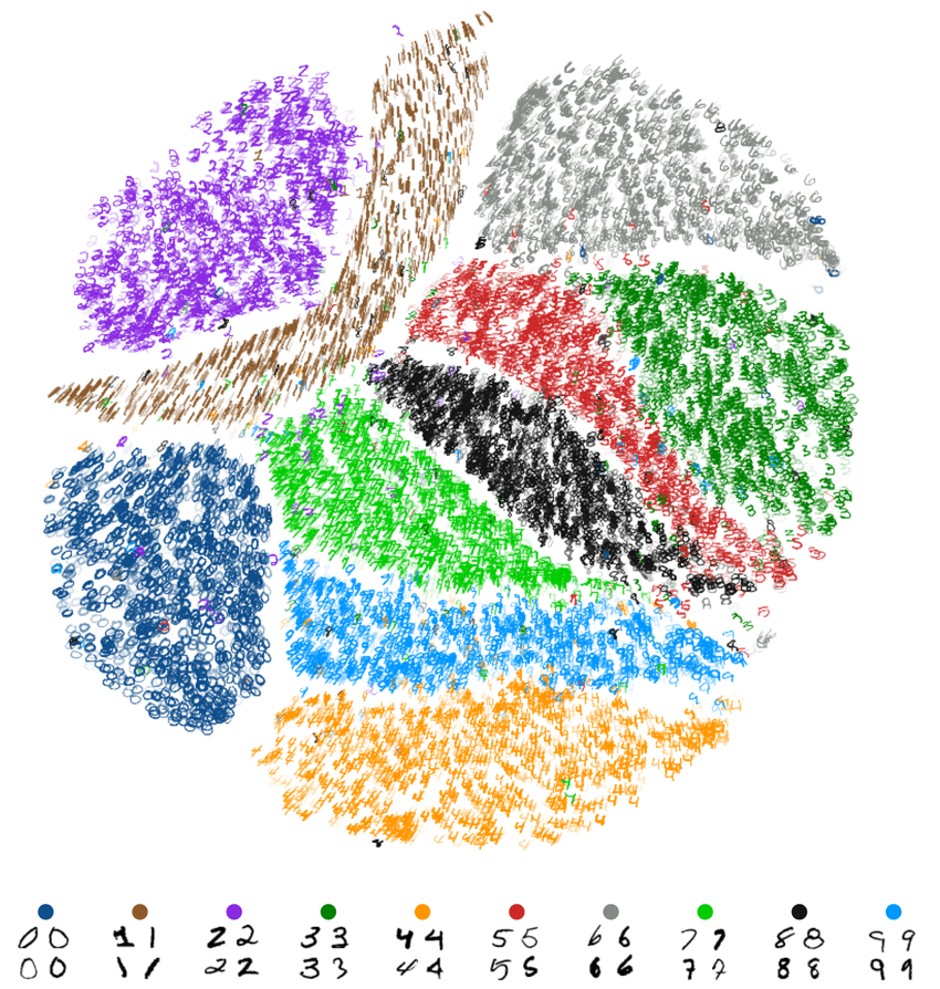
Fig. 1.9 t-SNE algorithm applied on MNIST dataset constaining pictures of handwritten digits. Picture from [Pezzotti, 2019]

1.2.4.1.2. Supervised learning

Supervised learning difference is that users give learning information (variable to explain) to learn in the right way. Most of predictive models are from this category. Indeed, the value to predict (variable, class, etc.) is the variable to explain and others are explanatory variables. From the informations given by the user, the model will adjust this parameters to fit to data and reduce the error of prediction on the train dataset. Regression models try to estimate the relationship between variables when classification models try to estimate the category of the individuals (Figure 1.10).

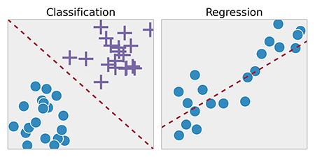
Fig. 1.10 Difference between classification and regression. Picture from Openclassrooms

Here, our problematic can be considered as a classification problem, that why we used classification methods on our data. Among classification algorithms, there are several kind of techniques which differ by their intern problem modelization. Tree based algorithms build or choose a decision tree from data identify classes from criterions on variables. Going down the tree permit to predict the class of an individual. There is many methods to build decision trees or choose the best randomly initialized tree (like Random Forest) (chapter 5 [Goodfellow et al., 2016]). Figure 1.11 show an example of classification/decision tree.

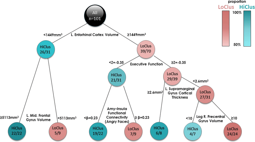
Fig. 1.11 Exemple of classification tree. Picture from [Ben-Zion et al., 2020]

Others classification models like SVM try to draw a boundary between individuals on the large dimensional space (see Support Vector Machine), and others try estimate de probability distribution of data classes, like Naive Baysian Classifier which use Bayesian law. Classification can also be made using Artificial Neural Netwok (ANN) (Figure 1.12). This type of method is a Reinforcement learning technique, i.e. that the algorithm will adjust parameters and end values for each time data go through the network. Also called Deep learning, there are many types of ANN structure and quantity of parameter can be huge, that allows models to learn deeply (part 2 [Goodfellow et al., 2016]).

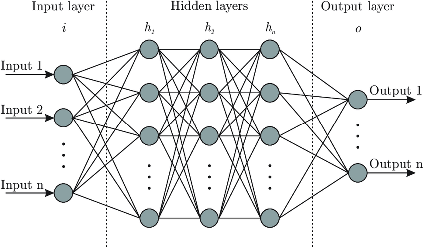
Fig. 1.12 Artificial neural network structure. Picture from [Bre et al., 2018]

This differents kind of techniques of classification has been tested on our data and will be show and discuss in section Pixel classification and Artificial Neural Network classifiers.

1.2.4.2. Classification evaluation

    To evaluate the quality of a classification model, there is multiple tools. Prime, a good practice in machine learning is to split dataset into train and test dataset. We will train the model on the train set and evaluate it on the test set making a prediction and comparing the true labels. Next we will look at 4 main learning statistics to estimate the model’s efficiency. Our problem being a binary classifcation problem, these formulas correspond to this kind of classification with negative and positive classes. True Positive (TP) correspond to the number of individals which have been predicted as positive class and have a positive true label. Same thing for True Negative (TN) that are negative individuals well predicted. False Positive (FP) is the number of individuals predicted as positive but are actually negative and vice versa for False Negative (FN).

• Accuracy is the most common metric score which correspond to the portion of good prediction, i.e. :

\[ \frac{TP + TN}{TP + TN + FP + FN} \]

• Precision is the proportion of predicted positive individals which are truely positive :

\[ \frac{TP}{TP + FP} \]

• Recall correspond to the True Positive Rate (TPR), i.e. the proportion of positive individuals classified correctly :

\[ \frac{TP}{TP + FN} \]

• Specificity is the True Negative Rate (TNR), the proportion of negative individuals classified as well :

\[ \frac{TN}{TN + FP} \]

These ratio allow us to evaluate the predictions of a model and adjust the parameters and hyperparameters. A popular visualization of a model score is ROC curve (Receiver Operating Characteristic). The idea is to place a model reporting as the TPR (recall or sensitivity) and the False Positive Rate (FPR), i.e. \(1-Specificity\). The Figure 1.13 present how to read a ROC curve. More the potition of the model’s curve or point is far of the \(x=y\) line, better is the classifier.

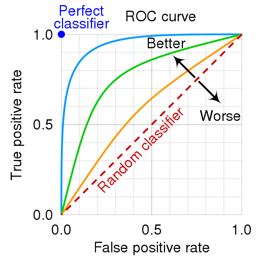
Fig. 1.13 Exemple of ROC curve with interpretive help. Picture from wikimedia

1.2.4.3. Python tools

    Scikit-learn Python package [Pedregosa et al., 2011] contains all tools we needed to apply classification models which dont use ANN. It also contains function to calculate learning metrics. Combinding this with matplotlib for figures, numpy for array manipulation, pandas and xarray for dataset manipulation, Scikit-learn allows the user to build a machine learning pipeline using Python kernel with a good computing optimization.

    For ANN models, we used Pytorch Python package [Paszke et al., 2019] to build differents models of ANN (see Artificial Neural Network classifiers) with flexibility and good performance on every device.