2.1. Experimental Data

2.1.1. AITA data : orientations and microstructure

    Orientaion maps obtained by the AITA is the initial data source that will use. Two thin sections have been made, one before and one after deformation.

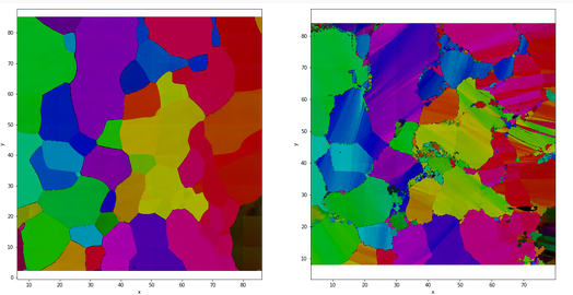
Fig. 2.1 Sample CI04 before and after creep colored by orientation of \(c\)-axis

    On the Figure 2.1 representing the map of orientations before and after deformation, we can observe germination of disoriented new grains resulting from the dynamic recrystallization process (see RX map : variable to explain). From those maps, it is possible to segment the microstructure and delimit grains and boundaries. After experiments, the results of 5 samples are good enough (clear microstructure, no breaks, no missing values) to be used in this study. Figure 2.2 shows the microstructure and the orientations of \(c\)-axes for the 5 samples.

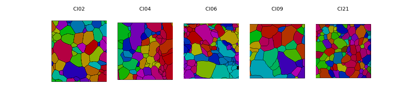
Fig. 2.2 Orientations of \(c\)-axes and grain boundaries of samples CI02, CI04, CI06, CI09, CI21

    This 5 experiments have not beeing done explicitly for this study, so there is some differences between the samples which should be considered as a potential bias. The main differences are that mean grain size is not the same and the final deformation strain is different too. The proportion of recrystallization is also different. This could have an impact on the classification and the analysis. The Table 2.1 show a simple description of the 5 samples. We can see that RX classes will be very unbalanced because of the low RX proportion.

Sample	Number of grains	Mean Size of grains (px)	Std of size of grains (px)	RX proportion (%)	Final deformation proportion (%)
CI02	\(72\)	\(3553\)	\(4398\)	\(4.48\)	\(3.0\)
CI04	\(86\)	\(3440\)	\(4469\)	\(10.23\)	\(5.5\)
CI06	\(144\)	\(2116\)	\(4112\)	\(5.05\)	\(3.7\)
CI09	\(43\)	\(6831\)	\(7547\)	\(5.71\)	\(6.0\)
CI21	\(121\)	\(2708\)	\(2567\)	\(6.69\)	\(3.4\)

Tab 2.1 : Global statistics of the 5 samples.

2.1.2. Data Computing : Geometric variables

    Orientations of \(c\)-axes have a characteristic which lead to a computational problem. \(c\) the \(c\)-axis , normal to the basal plane of the crystal, is a vector but direction have no sense here. Indeed, a plane normal to \(c\) and a plane normal to \(-c\) will have the same orientation. Using polar coordinates, \(\theta \in [0; 2\pi]\) and \(\phi \in [0;\pi]\) (see Figure 1.7 (right)) because 2 planes with \(c = (\phi,\theta)\) and \(c' = (\phi+\pi,\theta)\) will be identical but their representation is discontinue. With a view to describe experiments with scalar values due to \(c\)-axes, it is possible to compute several “geometrical” variables from maps of orientations. The idea is to calculate for each pixel a value explainable by the microstructure geometry.

2.1.2.1. Distance to grain boundary and triple junction

    Prime, we can calculate for each pixel the distance to the nearest grain boundary (dist2GB). Indeed, germination often occurs next to grain boundaries and triple junctions (see Recrystallisation). That’s why we also calculated for each pixel the distance to the nearest triple junction (dist2TJ). Functions to calculate these distances are implemented in xarrayaita.

2.1.2.2. Schmid factor

    Using \(c\)-axes orientations, we can compute the Schmid factor for each grain, that is a geometrical coefficient in relation to the angle \(\alpha\) between \(c\)-axix and the compression direction \(\sigma\) (Figure 2.3). Schmid factor is definied by :

\[ f(\alpha) = |cos(\alpha)sin(\alpha)| = |\frac{1}{2}sin(2\alpha)| \]

When compression is applied on axe \((Oy)\), there is the relation between \(\alpha\) and \((\phi,\theta)\) :

\[ cos(\alpha) = |sin(\phi)sin(\theta)| \]

Schmid factor with polar coordinates is so defined by :

\[ f(\phi,\theta) = |sin(\phi)sin(\theta)|\sqrt{1-sin^2(\phi)sin^2(\theta)} \]

The value of schmid factor is associated to pixels following their orientation.

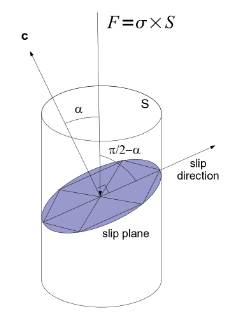
Fig. 2.3 Schmid cylinder. Picture from [Grennerat, 2011]

2.1.2.3. Schmid difference and misorientation angle

    To understand what append on grain boundaries, we can compare \(c\)-axes and Schmid factor. We calculated for each pixel the schmid difference (diff_schmid) at the closest grain boundary, i.e. :

\[ df((\phi _1,\theta _1),(\phi _2,\theta _2)) = |f(\phi _1,\theta _1) - f(\phi _2,\theta _2)| \]

with \((\phi _1,\theta _1)\) the \(c\)-axis orientation of the grain of the pixel and \((\phi _2,\theta _2)\) the \(c\)-axis orientation of the nearest grain.

    We also calculated the misorientation angle (mis_angle) between the \(c\)-axes \(c_1\) and \(c_2\) of two neighbor grains. The mis_angle \(\beta\) is difined by:

\[ \beta = Min(\beta _1,\beta _2) \]

with

\[\begin{split} cos(\beta _1) = c_1.c_2 \\ cos(\beta _2) = c_1.-c_2 \end{split}\]

Figure 2.4 represents the 5 maps corresponding to the distance to grain boundary, the distance to triple junction, the Schmid factor, the Schmid factor difference and misorientation angle values for each pixel.

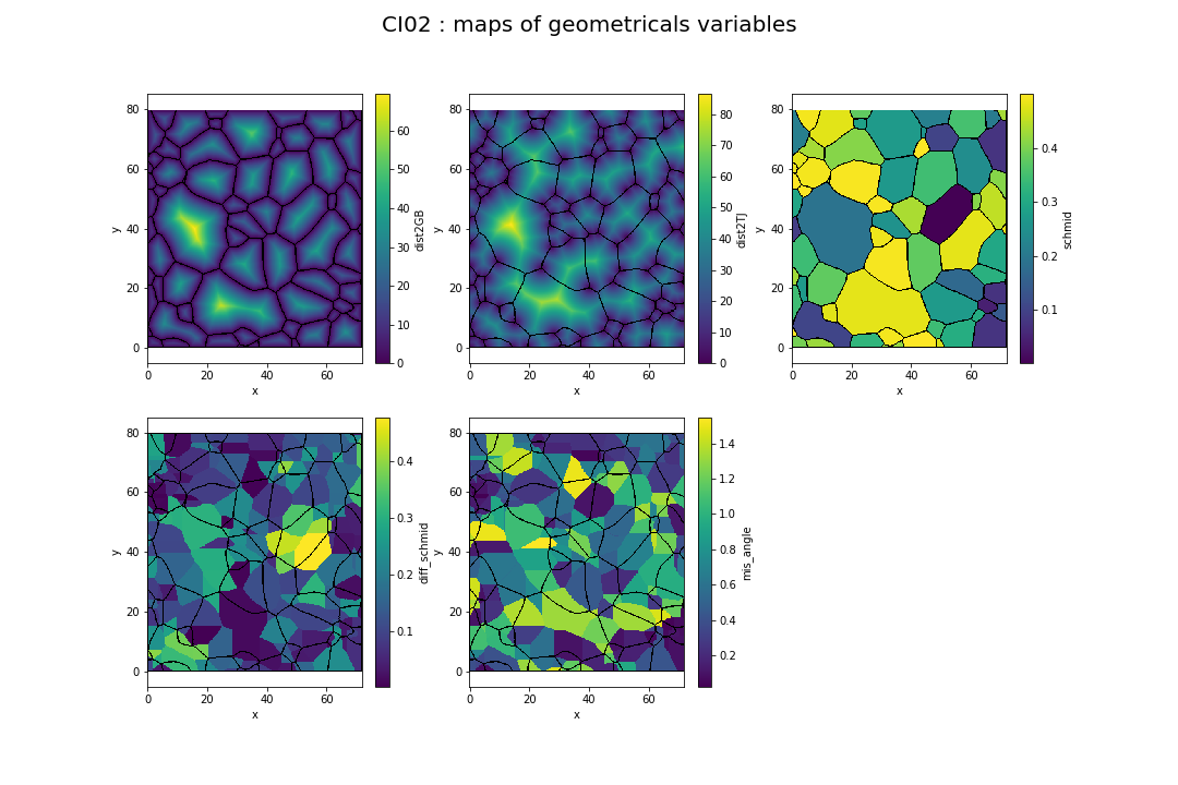
Fig. 2.4 Distance to GB, Distance to TJ, schmid factor, schmid difference and misorientation angle of experiment CI02

    Theses variables are resulting from AITA data computing. A python package to work with AITA data has been developed by Thomas Chauve. The package xarrayaita allows users to easily work with AITA data and also compute values of variables of Figure 2.4 using xarray.

2.1.3. CraFT data : Strain/Stress modelization

    Using the CraFT model presented in section Experimental tools, it is possible to simulate strain and stress fields from \(c\)-axes orientation’s map. In return of the model, we get for each pixel the stress tensor \(\sigma\) and the strain tensor \(\varepsilon\) :

\[\begin{split} \sigma = \begin{pmatrix} \sigma _{11} & \sigma _{12} & \sigma _{13}\\ \sigma _{12} & \sigma _{22} & \sigma _{23}\\ \sigma _{13} & \sigma _{23} & \sigma _{33} \end{pmatrix} = \sigma _{ij} \end{split}\]

\[\begin{split} \varepsilon = \begin{pmatrix} \varepsilon _{11} & \varepsilon _{12} & \varepsilon _{13}\\ \varepsilon _{12} & \varepsilon _{22} & \varepsilon _{23}\\ \varepsilon _{13} & \varepsilon _{23} & \varepsilon _{33} \end{pmatrix} = \varepsilon _{ij} \end{split}\]

We calculated the map of equivalent strain field (eqStrain) and the map of equivalent stress field (eqStress) of initial orientations, defined by :

\[ \sigma ^{eq} = \sqrt{\frac{2}{3}\sum_i \sum_j \sigma _{ij}\sigma _{ij}} = \sqrt{\frac{2}{3}\sigma _{ij}\sigma _{ij}} \]

\[ \varepsilon ^{eq} = \sqrt{\frac{2}{3}\sum_i \sum_j \varepsilon _{ij}\varepsilon _{ij}} = \sqrt{\frac{2}{3}\varepsilon _{ij}\varepsilon _{ij}} \]

According to these 2 variables, the work applied is defined by :

\[ W = \frac{1}{2} \sum_i \sum_j \varepsilon _{ij} \sigma _{ij} = \frac{1}{2} \varepsilon _{ij} \sigma _{ij} \]

CraFT model is based on internal parameters called slip systems. We can extract 2 intern parameters from this model corresponding to the prismatic activity (act_pr) and the pyramidal activity (act_py), meaning slipping activity in other planes that basis (see Figure 1.3). Finally, we obtain 5 variables extract from modelization that we can use for the classification problem. This 5 variables values are presented for CI02 on Figure 2.5.

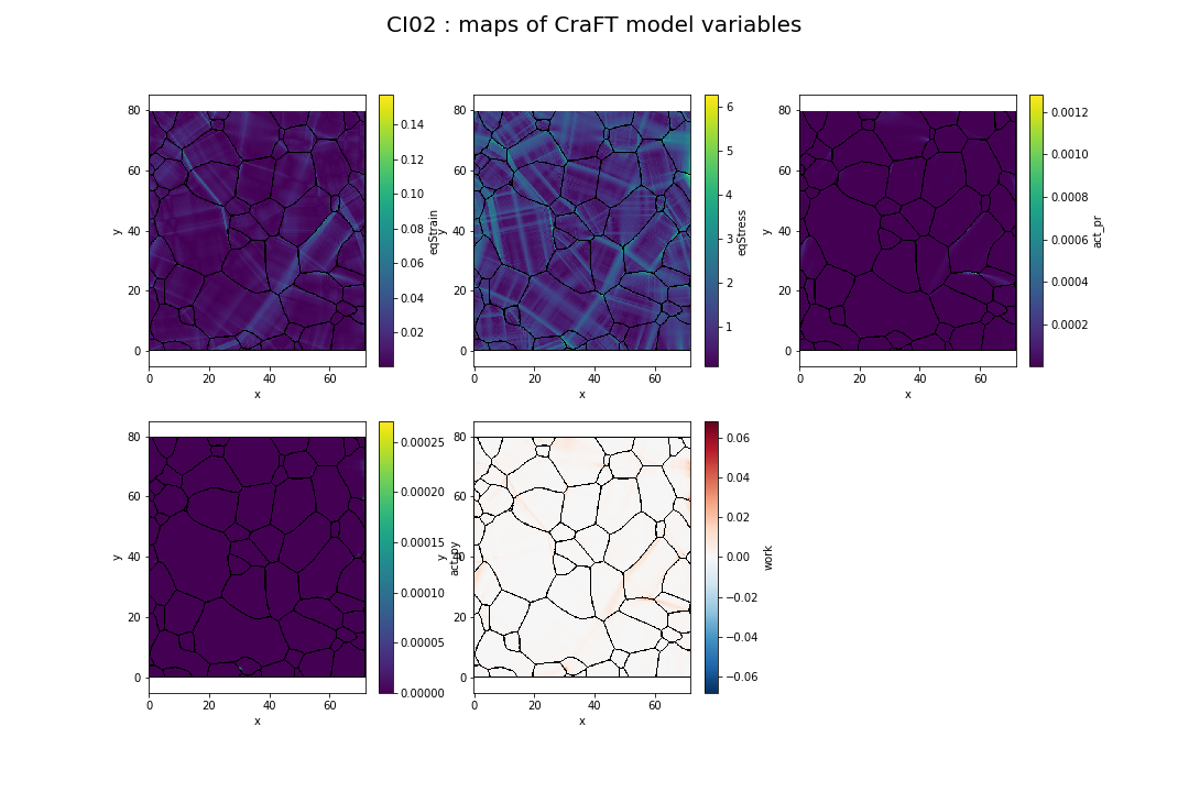
Fig. 2.5 Equivalent strain, equivalent stress, prismatic activity, pyramidal activity and work of experiment CI02

2.1.4. RX map : variable to explain

    Recall that we wanted to predict the positions of new ice crystals. Using AITA data of the end of the experiment (Figure 2.2), we are able to identify which grain wasn’t already there at the beginning. RX or Y is a binary variable which will be the class to predict, representing if a pixel take part of a recrystallized area or not. By cross correlations between initial and final orientations map, it is possible to make a projection of recrystallized grain positions on the initial picture. The Figure 2.6 shows the projection of RX grain positions extracted from the final AITA measurement on the initial microstructure obtain using the initial AITA analysis of CI02 experiment. We can observe that RX pixels are mostly next to grains boundary as it should be because RX append on grain boundary even if some points are a sometimes a little bit shifted. The global projection seems to be enough to consider it as an initial area of germination.

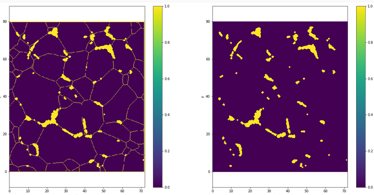
Fig. 2.6 RX projection on initial microstucture of CI02 experiment

    Initial dataset is so composed of 11 mapped variables for each experiment. In the first part of this report, we will consider each pixel as one individual with 10 explainable variables and 1 class (variable to explain). Computing pixels of all 5 pictures, we have a population of \(1 477 842\) individuals. Table 2.2 shows a part of the dataset for CI02 experiment.

	Y	dist2GB	dist2TJ	schmid	diff_schmid	misangle	eqStrain	eqStress	act_pr	act_py	work
0	0	0.0	1.0	0.395254	0.103993	0.391022	0.015412	2.344376	4.531981e-06	1.011138e-06	0.003950
1	0	0.0	0.0	0.395254	0.103993	0.391022	0.016234	2.400504	4.607910e-07	1.237610e-06	0.003692
2	0	0.0	1.0	0.395254	0.103993	0.391022	0.009668	2.570231	1.110663e-06	9.871840e-08	0.001585
3	0	0.0	2.0	0.395254	0.103993	0.391022	0.013143	2.546861	1.274664e-06	9.265364e-09	0.001447
4	0	0.0	3.0	0.395254	0.103993	0.391022	0.013521	2.653873	8.023945e-07	3.393400e-11	0.001319
...	...	...	...	...	...	...	...	...	...	...	...
255835	0	0.0	3.0	0.432296	0.033262	0.252094	0.009866	0.702662	1.342906e-06	2.662732e-13	0.000779
255836	0	0.0	2.0	0.432296	0.033262	0.252094	0.005627	0.740925	1.315377e-06	6.788590e-13	0.000375
255837	0	0.0	1.0	0.432296	0.033262	0.252094	0.005517	1.467539	1.497212e-06	1.407731e-14	0.000479
255838	0	0.0	0.0	0.432296	0.033262	0.252094	0.010359	1.968252	1.425730e-06	2.844993e-10	0.000894
255839	0	0.0	1.0	0.432296	0.033262	0.252094	0.014877	1.612373	1.132847e-06	7.408479e-11	0.001206

255840 rows × 11 columns

Tab 2.2 : Head and queue of initial CI02 dataset