2.2. Additional data

2.2.1. Data computing : Anisotropy factors of triple jonctions

    Data exposed in section Experimental Data have already been calculated before the begining of the internship by Thomas. We will see in section Data exploration that were not enought “spaced” in the variable space. Indeed, a probleme that occurs many times and affect the difficulty of the classification is that for situations as well as represented Figure 2.7, some pixels with a certain symmetry with respect to a grain boundary can have mostly same value for every variable exept Craft data which are not enough to dissociate them.

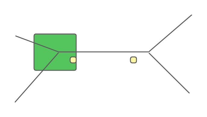
Fig. 2.7 Exemple of situation where for the two yellow pixels, dist2GB and dist2TJ have same value for both. Schmid factor is also the same beacuse they are from same grain. In addition, the nearest grain boundary is the same, involving that diff_schmid and mis_angle will also have same value. But the left pixel take part of a RX zone (green) whereas the right pixel is not recrystallized.

    In this kind of situation, we wanted to add variable that characterize the nearest triple junction (TJ). With the orientations of the 3 grains composing a triple junction, it is possible to characterize the shape of the TJ using the anisotropy factors calculated from the eigen values of the second order orientation tensor (OT2) \(M\) defined by :

\[ M = \sum_{i = 1}^{3} c_i \otimes c_i \]

with \(c_1\), \(c_2\) and \(c_3\) the \(c\)-axis of the 3 grains and

\[\begin{split} c \otimes c = \begin{pmatrix} c_xc_x & c_xc_y & c_xc_z\\ c_xc_y & c_yc_y & c_yc_z\\ c_xc_z & c_yc_z & c_zc_z \end{pmatrix} \end{split}\]

The 4 anisotropy factors are difined from the proper values of the OT2. Formulas are presented on Table 2.3

Name	Mathematical expression	Sphere shape	Needle Shape	Penny shape
		\((\mu _1 = \mu _2 = \mu _3)\)	\((\mu _1 << \mu _2 = \mu _3)\)	\((\mu _1 = \mu _2 >> \mu _3)\)
Relative anisotropy	\(std(\mu _i)/mean(\mu _i)\)	\(0\)	\(2.45\)	\(1.22\)
Fractional anisotropy	\(std(\mu _i)/\sqrt{mean(\mu _i^2)}\)	\(0\)	\(0.82\)	\(0.58\)
Volume ratio anisotropy	\(1 - \mu _1\mu _2\mu _3/mean(\mu _i)^3\)	\(0\)	\(1\)	\(0\)
Flatness anisotropy	\(\mu _3/\mu _2\)	\(1\)	Undefined	\(0\)

Tab 2.3 : Various anisotropy factors and expected values for distinctive shapes. \(\mu _i\) correspond to proper values of the second order orientation tensor \(M\).

    To calculate these new variables reffering triple junctions, we needed to apply the following process :

1. Calculate the coordinates of each TJ and determinate which grains are around.

2. Calculate the distance of each pixel to each TJ.

3. Determinate the closest TJ and the 3 grains composing it.

4. Get orientations of the 3 grains and compute the OT2 then the anisotropy factors.

    Most of the tools needed for this data manipulations were not already developed. I added few new functions allowing this pipeline to be repeated into xarrayaita. Pipeline’s notebook is here. Finally, we get the maps of the 4 anisotropy factors reffering to the nearest TJ represented Figure 2.8 for sample CI02. this 4 new variables have been added to the initial dataset with hope to fix simillarities problem (see Data exploration).

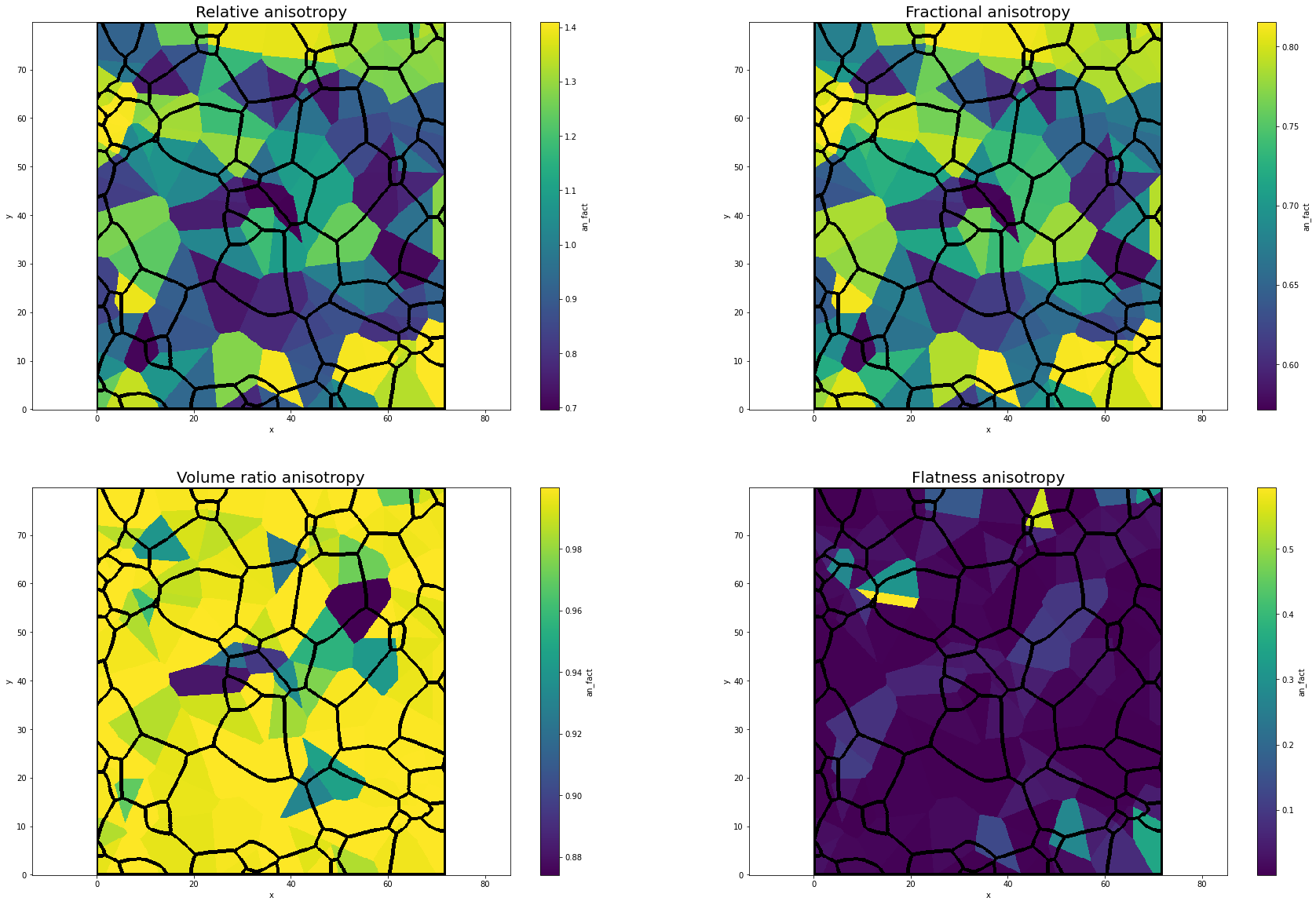
Fig. 2.8 Maps of anisotropy factors refering to the nearest TJ for CI02 sample

2.2.2. Triple jonctions dataset for tabular data learning

    After the first results obtained on ininitial data, decided to change our classification strategy. Classification methods were not able to identify more than area around grain boundaries and triple junctions (see Pixel classification). Keeping in mind that nucleation occurs mostly at neighbourhood of triple junctions, we decided to classify only triple junction instead of pixels, i.e. identify which triple junction has recrystallized or not. To do that we had to adapt the dataset and compute variables corresponding to TJ. After getting the coordinates and the grains composing it of all triple junctions like in the previous section with xarrayaita (TJ_map) and filter TJ junction too close to border (\(10px\)), we were able to compute the following variables for each TJ:

• The 3 Schmid factors corresponding to each grain of the TJ.

• The 3 diff_schmid of the 3 grains boundaries

• The 3 mis_angle of the 3 grain boundaries

• The 4 anisotropy factors (at the end we conserve only 1 : Data exploration)

• The mean values of the 5 CraFT variables (eqStrain, eqStress, act_py, act_pr, work) in a circlular area of \(10 px\) range.

We added 2 more types of variables to this dataset :

• The distance to the nearset other TJ, to estimate the density of triple junctions in this area.

• The number of pixels composing each grain of the TJ, to compare TJ of big grains in relation to small grains.

    Finally, we had to decide when consider a TJ as recrystallized. We looked at the circular area of \(10px\) range around each TJ and count the number of recrystallized pixels. We choose to consider a TJ as recrystallized if the proportion of RX pixel is higher than \(10\%\) of the area because we can’t say that a it is recrystallized if there are only few parse pixels in the neighborhood of the TJ.

    The description of the samples looking at the TJ is presented in Table 2.3 and a part of the dataset of CI02 is presented Table 2.4. The computation pipeline is available here.

Sample	number of TJ	% of RX
CI02	\(103\)	\(37.8\)
CI04	\(145\)	\(45.5\)
CI06	\(216\)	\(25.9\)
CI09	\(60\)	\(35.0\)
CI21	\(198\)	\(36.4\)

Tab 2.3 : TJ sample description

	RX	schmid1	schmid2	schmid3	diff_schmid1	diff_schmid2	diff_schmid3	misangle1	misangle2	misangle3	relative_an	eqStrain	eqStress	act_pr	act_py	work	dist1neigh	nb_pix_g1	nb_pix_g2	nb_pix_g3
0	0.0	0.419063	0.327499	0.491951	0.072887	0.091564	0.164451	1.454129	1.171702	1.165820	0.997188	0.004777	2.180479	1.901662e-06	3.912340e-09	0.000861	28.844410	419.0	2089.0	1546.0
1	0.0	0.499503	0.419063	0.491951	0.007553	0.072887	0.080440	1.171702	0.114888	1.286440	0.999970	0.010396	1.277755	7.124668e-06	3.018874e-08	0.001725	6.708204	2213.0	419.0	1546.0
2	0.0	0.103737	0.425714	0.395254	0.030460	0.291516	0.321977	0.351442	0.406263	0.072496	0.999695	0.008478	1.335520	3.627632e-06	8.096054e-09	0.001261	21.023796	7445.0	1153.0	812.0
3	1.0	0.468876	0.499503	0.342796	0.030627	0.156708	0.126080	0.997705	1.152839	0.990150	0.998742	0.004828	1.055209	1.307748e-06	1.897301e-09	0.000667	8.246211	308.0	2213.0	1196.0
4	0.0	0.309628	0.468876	0.342796	0.126080	0.033168	0.159249	0.157292	0.943856	0.990150	0.984860	0.007199	1.158688	6.099184e-07	6.984362e-09	0.000709	8.246211	4054.0	308.0	1196.0
...	...	...	...	...	...	...	...	...	...	...	...	...	...	...	...	...	...	...	...	...
100	1.0	0.101558	0.352455	0.215788	0.250897	0.136667	0.114230	0.270632	0.585201	0.315096	0.999952	0.013723	1.513008	3.832023e-05	4.820975e-07	0.004412	1.414214	3599.0	4667.0	2696.0
101	1.0	0.101558	0.352455	0.215788	0.136667	0.114230	0.250897	0.270632	0.585201	0.315096	0.999952	0.011586	1.663743	4.358300e-05	1.082345e-06	0.004974	1.414214	3599.0	4667.0	2696.0
102	0.0	0.076356	0.206418	0.432296	0.355940	0.130062	0.225878	0.581787	0.241980	0.350854	0.997504	0.007621	1.442819	4.854863e-07	9.044121e-09	0.000769	21.470911	5073.0	1112.0	396.0
103	0.0	0.478350	0.284126	0.378515	0.099836	0.194224	0.094389	0.647229	0.127852	0.538544	0.998606	0.022184	1.939872	2.352928e-06	1.961549e-06	0.004392	20.024984	5713.0	666.0	899.0
104	1.0	0.271630	0.284126	0.378515	0.094389	0.106885	0.012496	0.186720	0.127852	0.252362	0.999479	0.009972	1.753213	1.904186e-05	4.835008e-08	0.003018	25.317978	10830.0	666.0	899.0

103 rows × 20 columns

Tab 2.4 : CI02 TJ dataset head and queue

2.2.3. Triple jonctions dataset for convolutional and mixture Artificial Neural Network learning

In this same view to classify triple junctions, we made a third dataset structure made for Convolutional Neural Network (CNN) or others models which could use mapped variables. Instead of extract scalar variables for each TJ like we have done before, we defined a window \(10 \times 10 px\) sized, centered around the TJ. This new dataset is composed for each TJ by :

• The Schmid factor map \(10 \times 10 px\)

• The diff_schmid map \(10 \times 10 px\)

• The mis_angle map \(10 \times 10 px\)

• The eqStrain map \(10 \times 10 px\)

• The eqStress map \(10 \times 10 px\)

• The act_py map \(10 \times 10 px\)

• The act_pr map \(10 \times 10 px\)

• The work map \(10 \times 10 px\)

• The RX map \(10 \times 10 px\) used to define the RX class.

To define the RX class of each TJ, we decided to stay with the criterion according that :

\[\begin{split} RX = 1 \ if \ \sum_i \sum_j RX_{ij} > 10\% n \\ else \ RX = 0 \end{split}\]

with \(n\) the number of pixels in the window, here \(n=100\)

In addition to this 8 mapped variables used in Convolutional Neural Network, we added \(3\) scalar variables characterizing triple junction :

• One of the 4 anisotropy factors (volume ratio see Data exploration)

• The distance to the closest other TJ (Dtfn)

• The sum of the pixels composing grains of the TJ (sum_pix_g)

This variables will be used with the mapped variables in sec:mixture. The Figure 2.9 present the differenst variables of one TJ of sample CI02. The pipeline notebook to comptute these data is here.

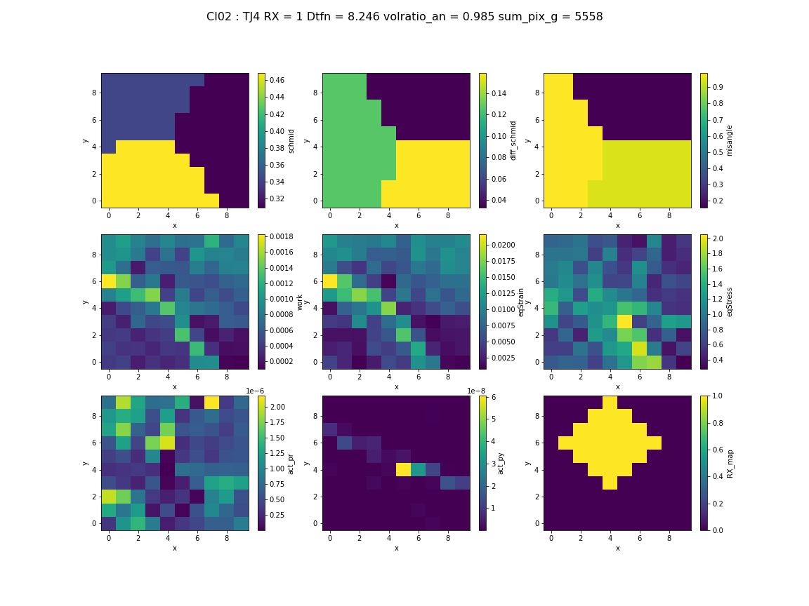
Fig. 2.9 A sample of the dataset CNN/Mixture NN models. Variables of TJ number 4 of sample CI02.