4.2. Artificial Neural Network classifiers

    We will now detail the results of the artificial neural network (ANN) models that we used to conclude the study of this data. Pipeline to use the ANN models with pytorch is available here

4.2.1. Convolutional Neural Network

    From this point, we used the last dataset we made for the convolutional learning (see Triple jonctions dataset for convolutional and mixture Artificial Neural Network learning). We built several neural architectures to learn on the 8 “mapped” variables we have, variating the number of channels and layers. The final model is presented Figure 4.4. After variating the hyperparameters, we got as “best” results the learning statistics presented Figure 4.5 and represented on ROC curve with a color map by epoch to observe the convergence of the model Figure 4.6. We chose to apply undersampling on data with rotation and symmetry of mapped variables to increase the number of observations and balance the number of TJ incoming from each sample. As we can see in the recall,specificity and accuracy curves, the dropout between train and test values happen very fast and test values seem to converge to values \(40 \%\) recall and \(60 \%\) specificity. Looking at the ROC curve, we can see that for some epochs, coordinates of points are below the \(x=y\) straight, indicating that the classification should be better if we switch labels of categories. This should have to effect on ROC curve by make a symmetry referring to the central point (0.5,0.5). In other terms, switching category in the situation where point is near to the \(x=y\) straight will not have an effect on this distance. That is why we leaved categories as predicted on the Figure 4.6. We can conclude to this classification that this model is not better that a random classifier, because all epochs and especially the last epochs are very close to the \(x=y\) straight.

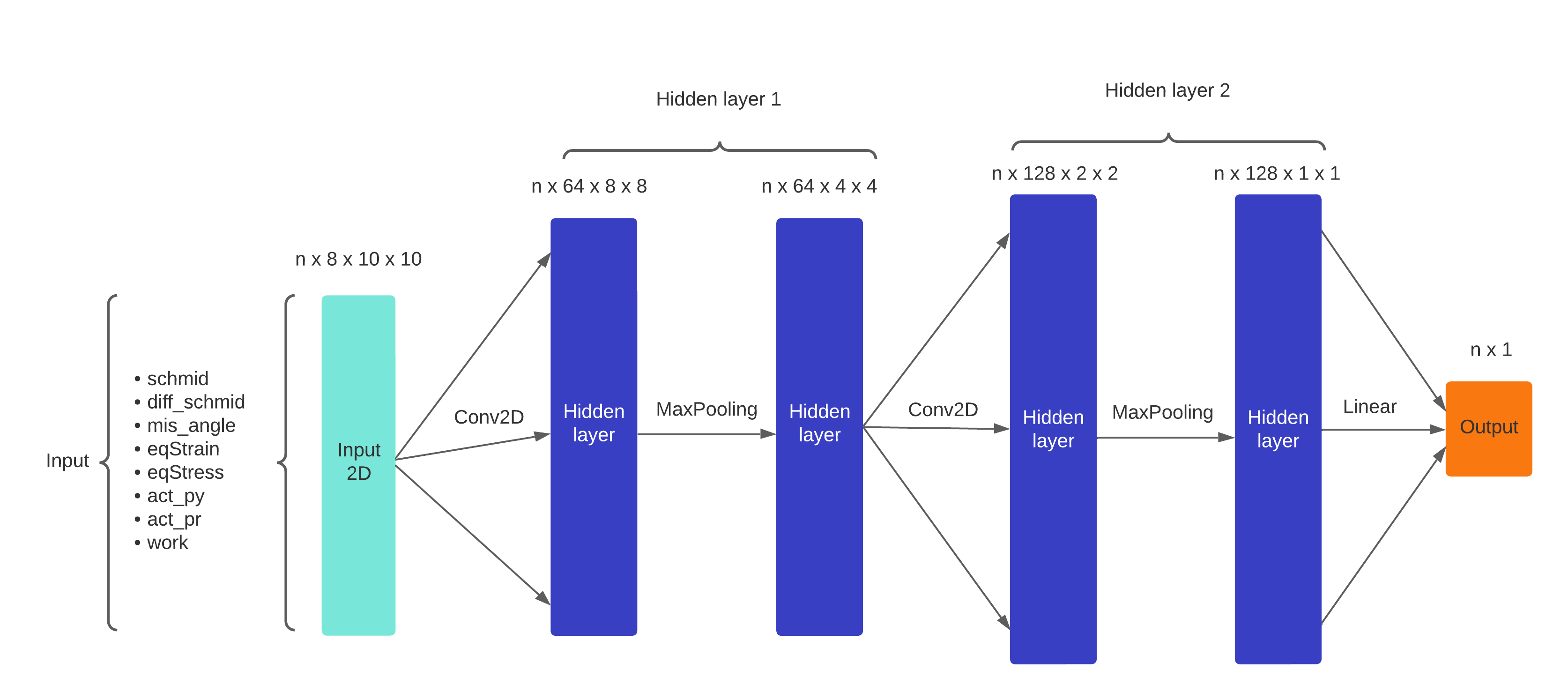
Fig. 4.4 CNN architecture also called CNet1

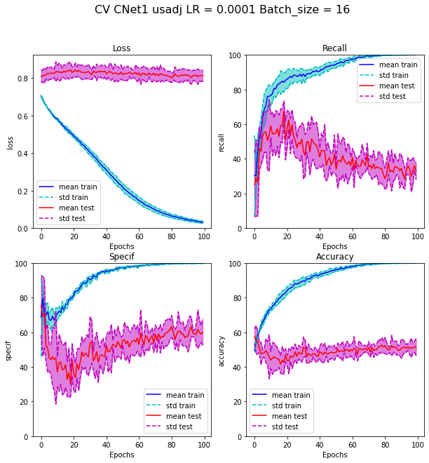
Fig. 4.5 Cross validation results of learning with CNet1 with undersampling adjusted method

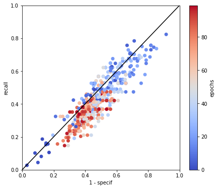
Fig. 4.6 ROC of the cross validation results of learning with CNet1 with undersampling adjusted method with coloration by epoch to enlight the convergence of the model.

4.2.2. Mixture Neural Network

    CNN being not able to well classify data with only the 8 mapped variables, we chose to build a neural architecture using these variables and also the variables referring to the TJ like anisotropy or distance to other TJ. I call this model a Mixture Neural Network. The architecture of the model is represented on Figure 4.7. After hyperparameters variation and modulation of channels and layers, we got the results presented in Figure 4.8 and Figure 4.9. We can see that the results are a little bit better, although that test loss function is still stuck, Indicating that the error in decision remains high on tests. But the variance of the cross validation values is too high to say that is really better.

    We try to limit the number of variable used to only the most important, to limit the number of parameters of the model, using only work,anisotropy factor and Schmid factor. The results of this reduced model are presented on Figure 4.10 and Figure 4.11. Unfortunately, results are not better. Variance of recall and specificity is huge because for some test set, network converges to a solution giving full zero or full one.

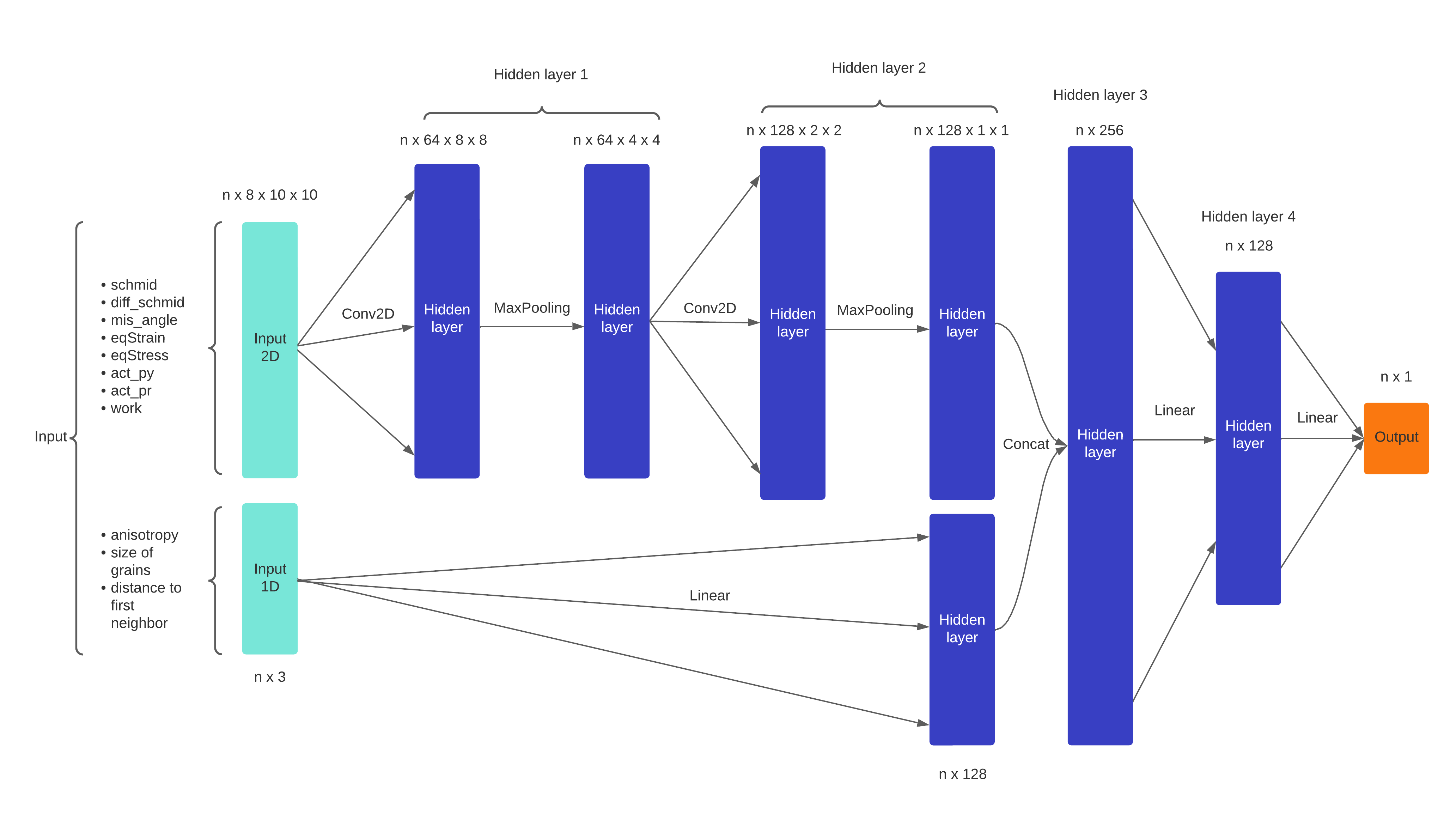
Fig. 4.7 Mixture NN architecture also called Net1

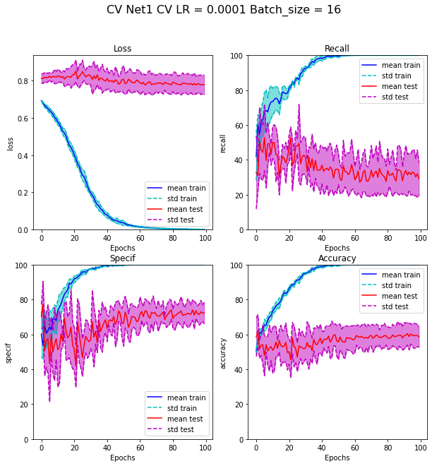
Fig. 4.8 Cross validation results of learning with Net1 with undersampling adjusted method

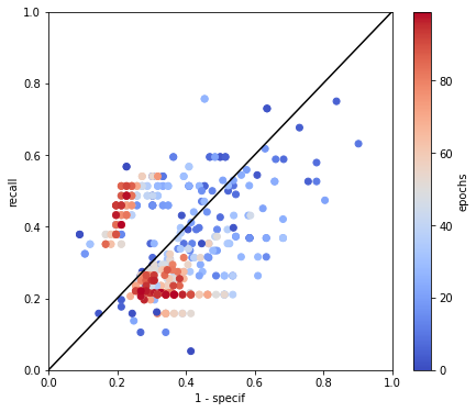
Fig. 4.9 ROC of the cross validation results of learning with Net1 with undersampling adjusted method with coloration by epoch to enlight the convergence of the model.

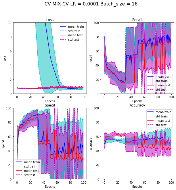
Fig. 4.10 Cross validation results of learning with minimal MIX model with undersampling adjusted method

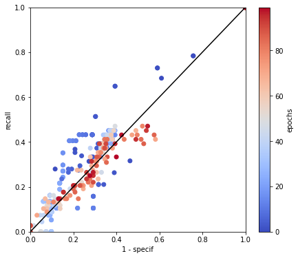
Fig. 4.11 ROC of the cross validation results of learning with minimal mixture model with undersampling adjusted method with coloration by epoch to enlight the convergence of the model.