Principal Components Analysis (PCA) on pixel dataset (with anisotropy)
Contents

Machine Learning to predict location of ice recrystallizationMay - July 2022 UGA and IGE internship M1 Statistics and Data Sciences (SSD) Renan MANCEAUX Supervisor : Thomas CHAUVE Dimensional Reduction |
8.4. Principal Components Analysis (PCA) on pixel dataset (with anisotropy)#
Exploration process before apply machine learning to craft data. Linear reduction of dimensions based on “least square” algorithm and projection into easyer representativ space made by linear combinations of variables.
8.4.1. Import packages#
import matplotlib.pyplot as plt
import numpy as np
import pandas as pd
import plotly.express as px
import seaborn as sns


import sys
sys.path.append("../../scripts/")
import utils


from sklearn.decomposition import PCA
8.4.2. Loading data#
CI02 = utils.load_data("../../data/for_learning_plus/CI02.npy")
CI04 = utils.load_data("../../data/for_learning_plus/CI04.npy")
CI06 = utils.load_data("../../data/for_learning_plus/CI06.npy")
CI09 = utils.load_data("../../data/for_learning_plus/CI09.npy")
CI21 = utils.load_data("../../data/for_learning_plus/CI21.npy")

CI02['batch'] = ['CI02'] * np.shape(CI02)[0]
CI04['batch'] = ['CI04'] * np.shape(CI04)[0]
CI06['batch'] = ['CI06'] * np.shape(CI06)[0]
CI09['batch'] = ['CI09'] * np.shape(CI09)[0]
CI21['batch'] = ['CI21'] * np.shape(CI21)[0]
8.4.3. PCA with anisotropy factors#
8.4.3.1. Variables selection#
data = pd.concat((CI02,CI04,CI06,CI09,CI21))
data['Y'] = data['Y'].astype(int)
data['batch'] = data['batch'].astype(object)
X = data.loc[:,((data.columns != 'Y')&(data.columns != 'batch'))]
y = data['Y']
b = data['batch']
8.4.3.2. Normalization#
norm_X = (X - X.mean())/X.std()
8.4.3.3. Apply PCA#
pca = PCA()
res_pca  = pca.fit(norm_X)
8.4.4. Results#
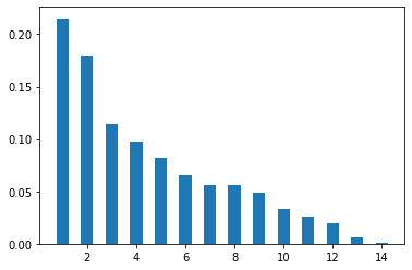
8.4.4.1. Eigen values / Explained variance ratio#
plt.bar(np.linspace(1,14,14),res_pca.explained_variance_ratio_,width=0.5)
plt.show()
8.4.4.2. First Principal plan of individuals#
components = pca.fit_transform(norm_X)

PCDf = pd.DataFrame(data = components
             , columns = ['PC 1', 'PC 2', 'PC 3', 'PC 4', 'PC 5','PC 6', 'PC 7', 'PC 8', 'PC 9', 'PC 10', 'PC 11', 'PC 12', 'PC 13', 'PC 14'])

colors_lab = {1:'red', 0 :'blue'}

colors_batch = {'CI02':'red', 'CI04':'green', 'CI06':'blue', 'CI09':'yellow', 'CI21':'black'}
# plt.figure(figsize=(8,8))
# plt.scatter(components.T[0],components.T[1],alpha=0.3,color = b.map(colors_batch))
# plt.xlabel(f"PC 1 ({(pca.explained_variance_ratio_[0] * 100):.1f}%)")
# plt.ylabel(f"PC 2 ({(pca.explained_variance_ratio_[1] * 100):.1f}%)")
# plt.title('first principal plan colored by batch')
# plt.show()
# plt.figure(figsize=(8,8))
# plt.scatter(components.T[0],components.T[1],alpha=0.3,color = y.map(colors_lab))
# plt.xlabel(f"PC 1 ({(pca.explained_variance_ratio_[0] * 100):.1f}%)")
# plt.ylabel(f"PC 2 ({(pca.explained_variance_ratio_[1] * 100):.1f}%)")
# plt.title('first principal plan colored by label')
# plt.show()
8.4.4.3. Individuals on 1-4 components#
# plt.figure(figsize=(10,10))
# plt.subplot(221)
# plt.scatter(components.T[0],components.T[1],alpha=0.3,color = b.map(colors_batch))
# plt.xlabel(f"PC 1 ({(pca.explained_variance_ratio_[0] * 100):.1f}%)")
# plt.ylabel(f"PC 2 ({(pca.explained_variance_ratio_[1] * 100):.1f}%)")
# plt.title('first principal plane colored by batch')

# plt.subplot(222)
# plt.scatter(components.T[2],components.T[3],alpha=0.3,color = b.map(colors_batch))
# plt.xlabel(f"PC 3 ({(pca.explained_variance_ratio_[2] * 100):.1f}%)")
# plt.ylabel(f"PC 4 ({(pca.explained_variance_ratio_[3] * 100):.1f}%)")
# plt.title('second principal plane colored by batch')

# plt.subplot(223)
# plt.scatter(components.T[0],components.T[1],alpha=0.3,color = y.map(colors_lab))
# plt.xlabel(f"PC 1 ({(pca.explained_variance_ratio_[0] * 100):.1f}%)")
# plt.ylabel(f"PC 2 ({(pca.explained_variance_ratio_[1] * 100):.1f}%)")
# plt.title('first principal plane colored by label')

# plt.subplot(224)
# plt.scatter(components.T[2],components.T[3],alpha=0.3,color = y.map(colors_lab))
# plt.xlabel(f"PC 3 ({(pca.explained_variance_ratio_[2] * 100):.1f}%)")
# plt.ylabel(f"PC 4 ({(pca.explained_variance_ratio_[3] * 100):.1f}%)")
# plt.title('second principal plane colored by label')

# plt.show()
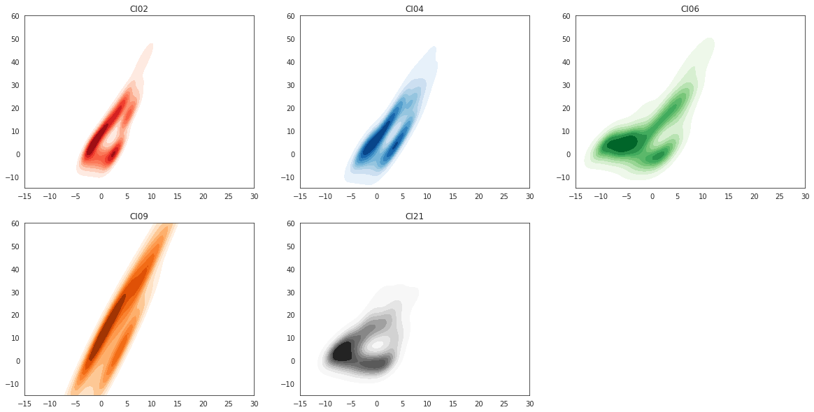
8.4.4.4. Density maps#
import warnings
warnings.filterwarnings('ignore')

df = PCDf[['PC 1','PC 2']]
df['batch'] = np.array(b)
df['RX'] = np.array(y)
CP_CI02 = df.where(df.batch=='CI02').dropna()
CP_CI04 = df.where(df.batch=='CI04').dropna()
CP_CI06 = df.where(df.batch=='CI06').dropna()
CP_CI09 = df.where(df.batch=='CI09').dropna()
CP_CI21 = df.where(df.batch=='CI21').dropna()
def filt(x,y, bins):
    x = np.array(x)
    y = np.array(y)

    d = np.digitize(x, bins)
    xfilt = []
    yfilt = []
    for i in np.unique(d):
        xi = x[d == i]
        yi = y[d == i]
        if len(xi) <= 2:
            xfilt.extend(list(xi))
            yfilt.extend(list(yi))
        else:
            xfilt.extend([xi[np.argmax(yi)], xi[np.argmin(yi)]])
            yfilt.extend([yi.max(), yi.min()])
    # prepend/append first/last point if necessary
    if x[0] != xfilt[0]:
        xfilt = [x[0]] + xfilt
        yfilt = [y[0]] + yfilt
    if x[-1] != xfilt[-1]:
        xfilt.append(x[-1])
        yfilt.append(y[-1])
    sort = np.argsort(xfilt)
    return np.array(xfilt)[sort], np.array(yfilt)[sort]
sns.set_style("white")
plt.figure(figsize=(20,10))
plt.subplot(231)

x = CP_CI02['PC 1']
y = CP_CI02['PC 2']
bins = np.linspace(x.min(),x.max(),301)
xf, yf = filt(x,y,bins)
sns.kdeplot(x=xf, y=yf, cmap="Reds", shade=True)
plt.xlim([-15,30])
plt.ylim([-15,60])
plt.title("CI02")

plt.subplot(232)

x = CP_CI04['PC 1']
y = CP_CI04['PC 2']
bins = np.linspace(x.min(),x.max(),301)
xf, yf = filt(x,y,bins)
sns.kdeplot(x=xf, y=yf, cmap="Blues", shade=True)
plt.xlim([-15,30])
plt.ylim([-15,60])
plt.title("CI04")

plt.subplot(233)

x = CP_CI06['PC 1']
y = CP_CI06['PC 2']
bins = np.linspace(x.min(),x.max(),301)
xf, yf = filt(x,y,bins)
sns.kdeplot(x=xf, y=yf, cmap="Greens", shade=True)
plt.xlim([-15,30])
plt.ylim([-15,60])
plt.title("CI06")

plt.subplot(234)

x = CP_CI09['PC 1']
y = CP_CI09['PC 2']
bins = np.linspace(x.min(),x.max(),301)
xf, yf = filt(x,y,bins)
sns.kdeplot(x=xf, y=yf, cmap="Oranges", shade=True)
plt.xlim([-15,30])
plt.ylim([-15,60])
plt.title("CI09")

plt.subplot(235)

x = CP_CI21['PC 1']
y = CP_CI21['PC 2']
bins = np.linspace(x.min(),x.max(),301)
xf, yf = filt(x,y,bins)
sns.kdeplot(x=xf, y=yf, cmap="Greys", shade=True)
plt.xlim([-15,30])
plt.ylim([-15,60])
plt.title("CI21")

plt.show()
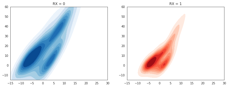
CP_y0 = df.where(df.RX==0).dropna()
CP_y1 = df.where(df.RX==1).dropna()
sns.set_style("white")
plt.figure(figsize=(20,10))
plt.subplot(231)

x = CP_y0['PC 1']
y = CP_y0['PC 2']
bins = np.linspace(x.min(),x.max(),301)
xf, yf = filt(x,y,bins)
sns.kdeplot(x=xf, y=yf, cmap="Blues", shade=True)
plt.xlim([-15,30])
plt.ylim([-15,60])
plt.title("RX = 0")

plt.subplot(232)

x = CP_y1['PC 1']
y = CP_y1['PC 2']
bins = np.linspace(x.min(),x.max(),301)
xf, yf = filt(x,y,bins)
sns.kdeplot(x=xf, y=yf, cmap="Reds", shade=True)
plt.xlim([-15,30])
plt.ylim([-15,60])
plt.title("RX = 1")

plt.show()
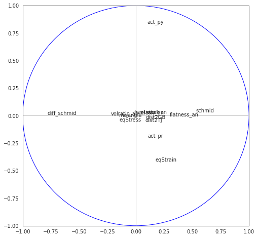
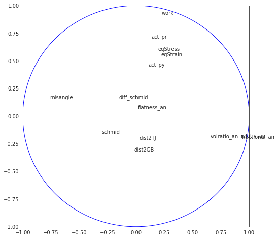
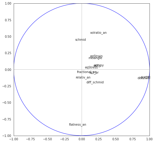
8.4.4.5. Correlation cirle on components 1-2, 3-4 and 5-6#
n = np.shape(norm_X)[0]
p = np.shape(norm_X)[1]
eigval = (n-1)/n*pca.explained_variance_
sqrt_eigval = np.sqrt(eigval)
corvar = np.zeros((p,p))
for k in range(p):
    corvar[:,k] = pca.components_[k,:] * sqrt_eigval[k]
fig, axes = plt.subplots(figsize=(8,8))
axes.set_xlim(-1,1)
axes.set_ylim(-1,1)

for j in range(p):
    plt.annotate(X.columns[j],(corvar[j,0],corvar[j,1]))

plt.plot([-1,1],[0,0],color='silver',linestyle='-',linewidth=1)
plt.plot([0,0],[-1,1],color='silver',linestyle='-',linewidth=1)
cercle = plt.Circle((0,0),1,color='blue',fill=False)
axes.add_artist(cercle)

plt.show()
fig, axes = plt.subplots(figsize=(8,8))
axes.set_xlim(-1,1)
axes.set_ylim(-1,1)

for j in range(p):
    plt.annotate(X.columns[j],(corvar[j,2],corvar[j,3]))

plt.plot([-1,1],[0,0],color='silver',linestyle='-',linewidth=1)
plt.plot([0,0],[-1,1],color='silver',linestyle='-',linewidth=1)
cercle = plt.Circle((0,0),1,color='blue',fill=False)
axes.add_artist(cercle)

plt.show()
fig, axes = plt.subplots(figsize=(8,8))
axes.set_xlim(-1,1)
axes.set_ylim(-1,1)

for j in range(p):
    plt.annotate(X.columns[j],(corvar[j,4],corvar[j,5]))

plt.plot([-1,1],[0,0],color='silver',linestyle='-',linewidth=1)
plt.plot([0,0],[-1,1],color='silver',linestyle='-',linewidth=1)
cercle = plt.Circle((0,0),1,color='blue',fill=False)
axes.add_artist(cercle)

plt.show()