Quick start
Warning
It is currently under devellopement. Please contact me before using it.
Load DICe output
DICe is an open source software to performe Digital Image Correlation.
adr_DICe='/data/Manips/Columnar_Ice/CI02/DIC_Analysis/1n_analysis/n16/'
import os
import numpy as np
import xarray as xr
import matplotlib.pyplot as plt
%matplotlib inline
import xarray_dic.loadDIC as ldDIC
import xarray_symTensor2d.xarray_symTensor2d as xT
import xarray_dic.xarray_dic as xd
ds=ldDIC.loadDICe(adr_DICe,0.01,10)
ds
<xarray.Dataset>
Dimensions:       (d: 2, sT: 6, time: 45, x: 96, xt: 95, y: 102, yt: 101)
Coordinates:
  * x             (x) float64 0.0 0.16 0.32 0.48 0.64 ... 14.72 14.88 15.04 15.2
  * y             (y) float64 0.0 0.16 0.32 0.48 0.64 ... 15.68 15.84 16.0 16.16
  * xt            (xt) float64 0.16 0.32 0.48 0.64 ... 14.72 14.88 15.04 15.2
  * yt            (yt) float64 0.16 0.32 0.48 0.64 ... 15.68 15.84 16.0 16.16
  * time          (time) float64 10.0 20.0 30.0 40.0 ... 420.0 430.0 440.0 450.0
Dimensions without coordinates: d, sT
Data variables:
    displacement  (time, y, x, d) float64 nan nan nan ... -0.8152 0.235 -0.8212
    strain        (time, yt, xt, sT) float64 nan nan nan nan ... nan nan nan nan
Attributes:
    unit_time:      seconds
    step_size:      0.01
    unit_position:  millimeter
    window_size:    16
    path_dat:       /data/Manips/Columnar_Ice/CI02/DIC_Analysis/1n_analysis/n16/
DIC_software: DICe- d: 2
- sT: 6
- time: 45
- x: 96
- xt: 95
- y: 102
- yt: 101
- x(x)float640.0 0.16 0.32 ... 14.88 15.04 15.2
array([ 0. , 0.16, 0.32, 0.48, 0.64, 0.8 , 0.96, 1.12, 1.28, 1.44, 1.6 , 1.76, 1.92, 2.08, 2.24, 2.4 , 2.56, 2.72, 2.88, 3.04, 3.2 , 3.36, 3.52, 3.68, 3.84, 4. , 4.16, 4.32, 4.48, 4.64, 4.8 , 4.96, 5.12, 5.28, 5.44, 5.6 , 5.76, 5.92, 6.08, 6.24, 6.4 , 6.56, 6.72, 6.88, 7.04, 7.2 , 7.36, 7.52, 7.68, 7.84, 8. , 8.16, 8.32, 8.48, 8.64, 8.8 , 8.96, 9.12, 9.28, 9.44, 9.6 , 9.76, 9.92, 10.08, 10.24, 10.4 , 10.56, 10.72, 10.88, 11.04, 11.2 , 11.36, 11.52, 11.68, 11.84, 12. , 12.16, 12.32, 12.48, 12.64, 12.8 , 12.96, 13.12, 13.28, 13.44, 13.6 , 13.76, 13.92, 14.08, 14.24, 14.4 , 14.56, 14.72, 14.88, 15.04, 15.2 ]) - y(y)float640.0 0.16 0.32 ... 15.84 16.0 16.16
array([ 0. , 0.16, 0.32, 0.48, 0.64, 0.8 , 0.96, 1.12, 1.28, 1.44, 1.6 , 1.76, 1.92, 2.08, 2.24, 2.4 , 2.56, 2.72, 2.88, 3.04, 3.2 , 3.36, 3.52, 3.68, 3.84, 4. , 4.16, 4.32, 4.48, 4.64, 4.8 , 4.96, 5.12, 5.28, 5.44, 5.6 , 5.76, 5.92, 6.08, 6.24, 6.4 , 6.56, 6.72, 6.88, 7.04, 7.2 , 7.36, 7.52, 7.68, 7.84, 8. , 8.16, 8.32, 8.48, 8.64, 8.8 , 8.96, 9.12, 9.28, 9.44, 9.6 , 9.76, 9.92, 10.08, 10.24, 10.4 , 10.56, 10.72, 10.88, 11.04, 11.2 , 11.36, 11.52, 11.68, 11.84, 12. , 12.16, 12.32, 12.48, 12.64, 12.8 , 12.96, 13.12, 13.28, 13.44, 13.6 , 13.76, 13.92, 14.08, 14.24, 14.4 , 14.56, 14.72, 14.88, 15.04, 15.2 , 15.36, 15.52, 15.68, 15.84, 16. , 16.16]) - xt(xt)float640.16 0.32 0.48 ... 14.88 15.04 15.2
array([ 0.16, 0.32, 0.48, 0.64, 0.8 , 0.96, 1.12, 1.28, 1.44, 1.6 , 1.76, 1.92, 2.08, 2.24, 2.4 , 2.56, 2.72, 2.88, 3.04, 3.2 , 3.36, 3.52, 3.68, 3.84, 4. , 4.16, 4.32, 4.48, 4.64, 4.8 , 4.96, 5.12, 5.28, 5.44, 5.6 , 5.76, 5.92, 6.08, 6.24, 6.4 , 6.56, 6.72, 6.88, 7.04, 7.2 , 7.36, 7.52, 7.68, 7.84, 8. , 8.16, 8.32, 8.48, 8.64, 8.8 , 8.96, 9.12, 9.28, 9.44, 9.6 , 9.76, 9.92, 10.08, 10.24, 10.4 , 10.56, 10.72, 10.88, 11.04, 11.2 , 11.36, 11.52, 11.68, 11.84, 12. , 12.16, 12.32, 12.48, 12.64, 12.8 , 12.96, 13.12, 13.28, 13.44, 13.6 , 13.76, 13.92, 14.08, 14.24, 14.4 , 14.56, 14.72, 14.88, 15.04, 15.2 ]) - yt(yt)float640.16 0.32 0.48 ... 15.84 16.0 16.16
array([ 0.16, 0.32, 0.48, 0.64, 0.8 , 0.96, 1.12, 1.28, 1.44, 1.6 , 1.76, 1.92, 2.08, 2.24, 2.4 , 2.56, 2.72, 2.88, 3.04, 3.2 , 3.36, 3.52, 3.68, 3.84, 4. , 4.16, 4.32, 4.48, 4.64, 4.8 , 4.96, 5.12, 5.28, 5.44, 5.6 , 5.76, 5.92, 6.08, 6.24, 6.4 , 6.56, 6.72, 6.88, 7.04, 7.2 , 7.36, 7.52, 7.68, 7.84, 8. , 8.16, 8.32, 8.48, 8.64, 8.8 , 8.96, 9.12, 9.28, 9.44, 9.6 , 9.76, 9.92, 10.08, 10.24, 10.4 , 10.56, 10.72, 10.88, 11.04, 11.2 , 11.36, 11.52, 11.68, 11.84, 12. , 12.16, 12.32, 12.48, 12.64, 12.8 , 12.96, 13.12, 13.28, 13.44, 13.6 , 13.76, 13.92, 14.08, 14.24, 14.4 , 14.56, 14.72, 14.88, 15.04, 15.2 , 15.36, 15.52, 15.68, 15.84, 16. , 16.16]) - time(time)float6410.0 20.0 30.0 ... 440.0 450.0
array([ 10.,  20.,  30.,  40.,  50.,  60.,  70.,  80.,  90., 100., 110., 120.,
       130., 140., 150., 160., 170., 180., 190., 200., 210., 220., 230., 240.,
       250., 260., 270., 280., 290., 300., 310., 320., 330., 340., 350., 360.,
       370., 380., 390., 400., 410., 420., 430., 440., 450.])
- displacement(time, y, x, d)float64nan nan nan ... 0.235 -0.8212
array([[[[ nan, nan], [ nan, nan], [ nan, nan], ..., [-1.4708e-02, -2.1862e-02], [-1.3753e-02, -2.0280e-02], [-1.4661e-02, -2.1506e-02]], [[ nan, nan], [-1.0475e-02, -2.5510e-02], [-1.0062e-02, -2.5738e-02], ..., [-1.4876e-02, -2.1282e-02], [-1.4427e-02, -2.1630e-02], [-1.4631e-02, -2.1781e-02]], [[ nan, nan], [-1.0518e-02, -2.5364e-02], [-1.0197e-02, -2.5803e-02], ..., ... ..., [ nan, nan], [ nan, nan], [ nan, nan]], [[-1.5693e-02, -8.9626e-01], [-1.7348e-02, -8.9149e-01], [-1.8040e-02, -8.8755e-01], ..., [ 2.3162e-01, -8.0600e-01], [ nan, nan], [ nan, nan]], [[-1.7283e-02, -8.9785e-01], [-1.9941e-02, -8.9472e-01], [-2.2196e-02, -8.8938e-01], ..., [ nan, nan], [ 2.3532e-01, -8.1522e-01], [ 2.3504e-01, -8.2124e-01]]]]) - strain(time, yt, xt, sT)float64nan nan nan nan ... nan nan nan nan
array([[[[            nan,             nan,             nan,
                      nan,             nan,             nan],
         [            nan,             nan,             nan,
                      nan,             nan,             nan],
         [            nan,             nan,             nan,
                      nan,             nan,             nan],
         ...,
         [-1.19391461e-03,  3.63212156e-03,             nan,
           2.47396625e-03,             nan,             nan],
         [ 2.81255283e-03, -8.39303172e-03,             nan,
          -3.19048488e-03,             nan,             nan],
         [-1.27374186e-03, -1.71725537e-03,             nan,
          -3.77433496e-04,             nan,             nan]],

        [[            nan,             nan,             nan,
                      nan,             nan,             nan],
         [ 2.01202660e-03, -4.05811523e-04,             nan,
          -1.79403906e-03,             nan,             nan],
         [-4.61848340e-04, -1.78488711e-03,             nan,
           1.23311262e-03,             nan,             nan],
...
         [            nan,             nan,             nan,
                      nan,             nan,             nan],
         [            nan,             nan,             nan,
                      nan,             nan,             nan],
         [            nan,             nan,             nan,
                      nan,             nan,             nan]],

        [[-1.62831667e-02, -1.98524112e-02,             nan,
           1.61527918e-03,             nan,             nan],
         [-1.34374878e-02, -1.10347415e-02,             nan,
           3.69217930e-03,             nan,             nan],
         [-3.75985107e-03,  5.57378625e-03,             nan,
           2.68127344e-03,             nan,             nan],
         ...,
         [            nan,             nan,             nan,
                      nan,             nan,             nan],
         [            nan,             nan,             nan,
                      nan,             nan,             nan],
         [            nan,             nan,             nan,
                      nan,             nan,             nan]]]])
- unit_time :
- seconds
- step_size :
- 0.01
- unit_position :
- millimeter
- window_size :
- 16
- path_dat :
- /data/Manips/Columnar_Ice/CI02/DIC_Analysis/1n_analysis/n16/
- DIC_software :
- DICe
Load 7D output
7D is a software to performe Digital Image Correlation written by Pierre Vacher.
adr_7d='/data/Manips/Columnar_Ice/CI23/DIC_Analysis/nm_analysis_0.5pc/n40/'
ds=ldDIC.load7D(adr_7d,0.01,0.005,unit_time='macro_strain')
ds
<xarray.Dataset>
Dimensions:       (d: 2, sT: 6, time: 11, x: 108, y: 108)
Coordinates:
  * x             (x) float64 0.0 0.4 0.8 1.2 1.6 ... 41.2 41.6 42.0 42.4 42.8
  * y             (y) float64 0.0 0.4 0.8 1.2 1.6 ... 41.2 41.6 42.0 42.4 42.8
  * time          (time) float64 0.005 0.01 0.015 0.02 ... 0.04 0.045 0.05 0.055
Dimensions without coordinates: d, sT
Data variables:
    displacement  (time, y, x, d) float64 -0.01382 0.02172 ... 0.05585 0.2646
    strain        (time, y, x, sT) float64 -0.0003503 0.009625 nan ... nan nan
Attributes:
    unit_time:      macro_strain
    step_size:      0.01
    unit_position:  millimeter
    window_size:    40
    path_dat:       /data/Manips/Columnar_Ice/CI23/DIC_Analysis/nm_analysis_0...
DIC_software: 7D- d: 2
- sT: 6
- time: 11
- x: 108
- y: 108
- x(x)float640.0 0.4 0.8 1.2 ... 42.0 42.4 42.8
array([ 0. , 0.4, 0.8, 1.2, 1.6, 2. , 2.4, 2.8, 3.2, 3.6, 4. , 4.4, 4.8, 5.2, 5.6, 6. , 6.4, 6.8, 7.2, 7.6, 8. , 8.4, 8.8, 9.2, 9.6, 10. , 10.4, 10.8, 11.2, 11.6, 12. , 12.4, 12.8, 13.2, 13.6, 14. , 14.4, 14.8, 15.2, 15.6, 16. , 16.4, 16.8, 17.2, 17.6, 18. , 18.4, 18.8, 19.2, 19.6, 20. , 20.4, 20.8, 21.2, 21.6, 22. , 22.4, 22.8, 23.2, 23.6, 24. , 24.4, 24.8, 25.2, 25.6, 26. , 26.4, 26.8, 27.2, 27.6, 28. , 28.4, 28.8, 29.2, 29.6, 30. , 30.4, 30.8, 31.2, 31.6, 32. , 32.4, 32.8, 33.2, 33.6, 34. , 34.4, 34.8, 35.2, 35.6, 36. , 36.4, 36.8, 37.2, 37.6, 38. , 38.4, 38.8, 39.2, 39.6, 40. , 40.4, 40.8, 41.2, 41.6, 42. , 42.4, 42.8]) - y(y)float640.0 0.4 0.8 1.2 ... 42.0 42.4 42.8
array([ 0. , 0.4, 0.8, 1.2, 1.6, 2. , 2.4, 2.8, 3.2, 3.6, 4. , 4.4, 4.8, 5.2, 5.6, 6. , 6.4, 6.8, 7.2, 7.6, 8. , 8.4, 8.8, 9.2, 9.6, 10. , 10.4, 10.8, 11.2, 11.6, 12. , 12.4, 12.8, 13.2, 13.6, 14. , 14.4, 14.8, 15.2, 15.6, 16. , 16.4, 16.8, 17.2, 17.6, 18. , 18.4, 18.8, 19.2, 19.6, 20. , 20.4, 20.8, 21.2, 21.6, 22. , 22.4, 22.8, 23.2, 23.6, 24. , 24.4, 24.8, 25.2, 25.6, 26. , 26.4, 26.8, 27.2, 27.6, 28. , 28.4, 28.8, 29.2, 29.6, 30. , 30.4, 30.8, 31.2, 31.6, 32. , 32.4, 32.8, 33.2, 33.6, 34. , 34.4, 34.8, 35.2, 35.6, 36. , 36.4, 36.8, 37.2, 37.6, 38. , 38.4, 38.8, 39.2, 39.6, 40. , 40.4, 40.8, 41.2, 41.6, 42. , 42.4, 42.8]) - time(time)float640.005 0.01 0.015 ... 0.05 0.055
array([0.005, 0.01 , 0.015, 0.02 , 0.025, 0.03 , 0.035, 0.04 , 0.045, 0.05 ,
       0.055])
- displacement(time, y, x, d)float64-0.01382 0.02172 ... 0.05585 0.2646
array([[[[-0.0138176 , 0.02172363], [-0.01269367, 0.01667236], [-0.01334625, 0.01440186], ..., [ 0.10404297, 0.10395996], [ 0.10484131, 0.10501465], [ 0.10544434, 0.10472656]], [[-0.01522213, 0.01732422], [-0.01540913, 0.01399414], [-0.01498169, 0.01441284], ..., [ 0.10421265, 0.10360229], [ 0.10390991, 0.10512207], [ 0.1048877 , 0.10512207]], [[-0.01673748, 0.01780273], [-0.01681585, 0.01567993], [-0.01620945, 0.01436646], ..., ... ..., [ 0.05506348, 0.26319592], [ 0.0549292 , 0.26423786], [ 0.05506836, 0.26406746]], [[ nan, nan], [ 0.0068755 , 0.26888802], [ 0.00852865, 0.27011887], ..., [ 0.05532104, 0.26495453], [ 0.05540283, 0.2654261 ], [ 0.0554126 , 0.26554352]], [[ nan, nan], [-0.01929932, 0.30371521], [-0.00242554, 0.3003447 ], ..., [ 0.05619141, 0.26459679], [ 0.05521484, 0.26542751], [ 0.05584961, 0.26460365]]]]) - strain(time, y, x, sT)float64-0.0003503 0.009625 nan ... nan nan
array([[[[-3.50349874e-04,  9.62528773e-03,             nan,
          -1.80607068e-03,             nan,             nan],
         [ 1.87318481e-03,  6.62416639e-03,             nan,
          -7.78798712e-05,             nan,             nan],
         [-5.29296813e-04, -1.24854778e-04,             nan,
           2.18693574e-04,             nan,             nan],
         ...,
         [-7.77722598e-05,  6.72160764e-04,             nan,
           1.28303189e-03,             nan,             nan],
         [ 2.08509131e-03, -1.70079205e-04,             nan,
           1.11463387e-03,             nan,             nan],
         [ 9.89774591e-04, -9.75468662e-04,             nan,
           2.54816969e-05,             nan,             nan]],

        [[-2.83982634e-04,  3.67443566e-03,             nan,
          -1.96263939e-03,             nan,             nan],
         [ 1.30781333e-03,  1.09543174e-03,             nan,
          -5.09590784e-04,             nan,             nan],
         [-5.84078138e-04, -4.11169640e-06,             nan,
           1.57794810e-03,             nan,             nan],
...
         [ 1.15511520e-03, -1.54172420e-03,             nan,
          -6.96854375e-04,             nan,             nan],
         [-3.48088914e-04, -2.59150728e-03,             nan,
          -6.05857756e-04,             nan,             nan],
         [ 1.08583318e-03,  8.78957042e-04,             nan,
           7.23363657e-04,             nan,             nan]],

        [[            nan,             nan,             nan,
                      nan,             nan,             nan],
         [ 4.31097373e-02, -7.81000406e-02,             nan,
           3.00260577e-02,             nan,             nan],
         [-5.50938203e-05, -6.76996037e-02,             nan,
           3.52105387e-02,             nan,             nan],
         ...,
         [ 8.44421913e-04, -2.16673798e-04,             nan,
           1.30847562e-04,             nan,             nan],
         [ 4.10129986e-04, -1.11063570e-03,             nan,
          -2.96394021e-04,             nan,             nan],
         [ 2.40789144e-03,  3.42831877e-03,             nan,
           9.04984598e-04,             nan,             nan]]]])
- unit_time :
- macro_strain
- step_size :
- 0.01
- unit_position :
- millimeter
- window_size :
- 40
- path_dat :
- /data/Manips/Columnar_Ice/CI23/DIC_Analysis/nm_analysis_0.5pc/n40/
- DIC_software :
- 7D
Load spam output
You should have all the vtk file in one folder sorted by time.
adr_data='/data/Manips/Columnar_Ice/CI23/DIC_Analysis/Test_spam/spamcor/'
#ds=ldDIC.loadSpam(adr_data,0.01,10*60,unit_time='seconds')
ds
<xarray.Dataset>
Dimensions:       (d: 2, sT: 6, time: 11, x: 108, y: 108)
Coordinates:
  * x             (x) float64 0.0 0.4 0.8 1.2 1.6 ... 41.2 41.6 42.0 42.4 42.8
  * y             (y) float64 0.0 0.4 0.8 1.2 1.6 ... 41.2 41.6 42.0 42.4 42.8
  * time          (time) float64 0.005 0.01 0.015 0.02 ... 0.04 0.045 0.05 0.055
Dimensions without coordinates: d, sT
Data variables:
    displacement  (time, y, x, d) float64 -0.01382 0.02172 ... 0.05585 0.2646
    strain        (time, y, x, sT) float64 -0.0003503 0.009625 nan ... nan nan
Attributes:
    unit_time:      macro_strain
    step_size:      0.01
    unit_position:  millimeter
    window_size:    40
    path_dat:       /data/Manips/Columnar_Ice/CI23/DIC_Analysis/nm_analysis_0...
DIC_software: 7D- d: 2
- sT: 6
- time: 11
- x: 108
- y: 108
- x(x)float640.0 0.4 0.8 1.2 ... 42.0 42.4 42.8
array([ 0. , 0.4, 0.8, 1.2, 1.6, 2. , 2.4, 2.8, 3.2, 3.6, 4. , 4.4, 4.8, 5.2, 5.6, 6. , 6.4, 6.8, 7.2, 7.6, 8. , 8.4, 8.8, 9.2, 9.6, 10. , 10.4, 10.8, 11.2, 11.6, 12. , 12.4, 12.8, 13.2, 13.6, 14. , 14.4, 14.8, 15.2, 15.6, 16. , 16.4, 16.8, 17.2, 17.6, 18. , 18.4, 18.8, 19.2, 19.6, 20. , 20.4, 20.8, 21.2, 21.6, 22. , 22.4, 22.8, 23.2, 23.6, 24. , 24.4, 24.8, 25.2, 25.6, 26. , 26.4, 26.8, 27.2, 27.6, 28. , 28.4, 28.8, 29.2, 29.6, 30. , 30.4, 30.8, 31.2, 31.6, 32. , 32.4, 32.8, 33.2, 33.6, 34. , 34.4, 34.8, 35.2, 35.6, 36. , 36.4, 36.8, 37.2, 37.6, 38. , 38.4, 38.8, 39.2, 39.6, 40. , 40.4, 40.8, 41.2, 41.6, 42. , 42.4, 42.8]) - y(y)float640.0 0.4 0.8 1.2 ... 42.0 42.4 42.8
array([ 0. , 0.4, 0.8, 1.2, 1.6, 2. , 2.4, 2.8, 3.2, 3.6, 4. , 4.4, 4.8, 5.2, 5.6, 6. , 6.4, 6.8, 7.2, 7.6, 8. , 8.4, 8.8, 9.2, 9.6, 10. , 10.4, 10.8, 11.2, 11.6, 12. , 12.4, 12.8, 13.2, 13.6, 14. , 14.4, 14.8, 15.2, 15.6, 16. , 16.4, 16.8, 17.2, 17.6, 18. , 18.4, 18.8, 19.2, 19.6, 20. , 20.4, 20.8, 21.2, 21.6, 22. , 22.4, 22.8, 23.2, 23.6, 24. , 24.4, 24.8, 25.2, 25.6, 26. , 26.4, 26.8, 27.2, 27.6, 28. , 28.4, 28.8, 29.2, 29.6, 30. , 30.4, 30.8, 31.2, 31.6, 32. , 32.4, 32.8, 33.2, 33.6, 34. , 34.4, 34.8, 35.2, 35.6, 36. , 36.4, 36.8, 37.2, 37.6, 38. , 38.4, 38.8, 39.2, 39.6, 40. , 40.4, 40.8, 41.2, 41.6, 42. , 42.4, 42.8]) - time(time)float640.005 0.01 0.015 ... 0.05 0.055
array([0.005, 0.01 , 0.015, 0.02 , 0.025, 0.03 , 0.035, 0.04 , 0.045, 0.05 ,
       0.055])
- displacement(time, y, x, d)float64-0.01382 0.02172 ... 0.05585 0.2646
array([[[[-0.0138176 , 0.02172363], [-0.01269367, 0.01667236], [-0.01334625, 0.01440186], ..., [ 0.10404297, 0.10395996], [ 0.10484131, 0.10501465], [ 0.10544434, 0.10472656]], [[-0.01522213, 0.01732422], [-0.01540913, 0.01399414], [-0.01498169, 0.01441284], ..., [ 0.10421265, 0.10360229], [ 0.10390991, 0.10512207], [ 0.1048877 , 0.10512207]], [[-0.01673748, 0.01780273], [-0.01681585, 0.01567993], [-0.01620945, 0.01436646], ..., ... ..., [ 0.05506348, 0.26319592], [ 0.0549292 , 0.26423786], [ 0.05506836, 0.26406746]], [[ nan, nan], [ 0.0068755 , 0.26888802], [ 0.00852865, 0.27011887], ..., [ 0.05532104, 0.26495453], [ 0.05540283, 0.2654261 ], [ 0.0554126 , 0.26554352]], [[ nan, nan], [-0.01929932, 0.30371521], [-0.00242554, 0.3003447 ], ..., [ 0.05619141, 0.26459679], [ 0.05521484, 0.26542751], [ 0.05584961, 0.26460365]]]]) - strain(time, y, x, sT)float64-0.0003503 0.009625 nan ... nan nan
array([[[[-3.50349874e-04,  9.62528773e-03,             nan,
          -1.80607068e-03,             nan,             nan],
         [ 1.87318481e-03,  6.62416639e-03,             nan,
          -7.78798712e-05,             nan,             nan],
         [-5.29296813e-04, -1.24854778e-04,             nan,
           2.18693574e-04,             nan,             nan],
         ...,
         [-7.77722598e-05,  6.72160764e-04,             nan,
           1.28303189e-03,             nan,             nan],
         [ 2.08509131e-03, -1.70079205e-04,             nan,
           1.11463387e-03,             nan,             nan],
         [ 9.89774591e-04, -9.75468662e-04,             nan,
           2.54816969e-05,             nan,             nan]],

        [[-2.83982634e-04,  3.67443566e-03,             nan,
          -1.96263939e-03,             nan,             nan],
         [ 1.30781333e-03,  1.09543174e-03,             nan,
          -5.09590784e-04,             nan,             nan],
         [-5.84078138e-04, -4.11169640e-06,             nan,
           1.57794810e-03,             nan,             nan],
...
         [ 1.15511520e-03, -1.54172420e-03,             nan,
          -6.96854375e-04,             nan,             nan],
         [-3.48088914e-04, -2.59150728e-03,             nan,
          -6.05857756e-04,             nan,             nan],
         [ 1.08583318e-03,  8.78957042e-04,             nan,
           7.23363657e-04,             nan,             nan]],

        [[            nan,             nan,             nan,
                      nan,             nan,             nan],
         [ 4.31097373e-02, -7.81000406e-02,             nan,
           3.00260577e-02,             nan,             nan],
         [-5.50938203e-05, -6.76996037e-02,             nan,
           3.52105387e-02,             nan,             nan],
         ...,
         [ 8.44421913e-04, -2.16673798e-04,             nan,
           1.30847562e-04,             nan,             nan],
         [ 4.10129986e-04, -1.11063570e-03,             nan,
          -2.96394021e-04,             nan,             nan],
         [ 2.40789144e-03,  3.42831877e-03,             nan,
           9.04984598e-04,             nan,             nan]]]])
- unit_time :
- macro_strain
- step_size :
- 0.01
- unit_position :
- millimeter
- window_size :
- 40
- path_dat :
- /data/Manips/Columnar_Ice/CI23/DIC_Analysis/nm_analysis_0.5pc/n40/
- DIC_software :
- 7D
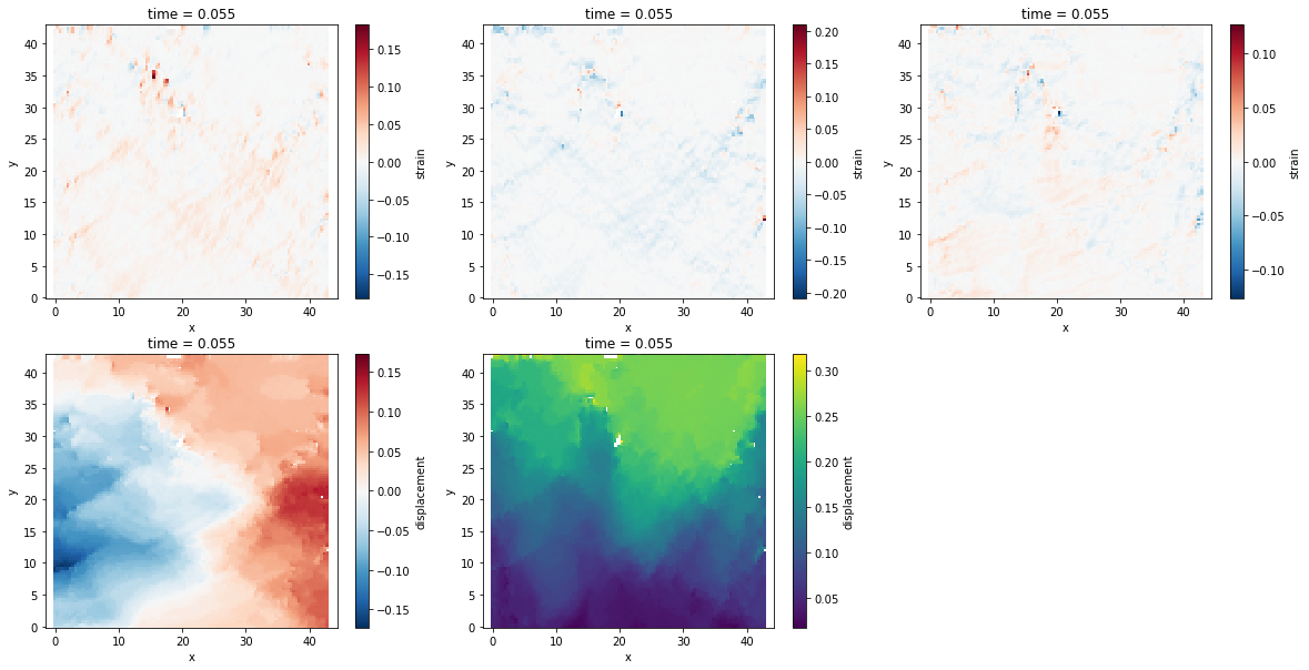
Visualize the data
To plot the strain field and displacement field for a given time step ts
ts=10
plt.figure(figsize=(20,10))
plt.subplot(231)
ds.strain[ts,:,:,0].plot()
plt.axis('equal')
plt.subplot(232)
ds.strain[ts,:,:,1].plot()
plt.axis('equal')
plt.subplot(233)
ds.strain[ts,:,:,3].plot()
plt.axis('equal')
plt.subplot(234)
ds.displacement[ts,:,:,0].plot()
plt.axis('equal')
plt.subplot(235)
ds.displacement[ts,:,:,1].plot()
plt.axis('equal')
(-0.2, 43.0, -0.2, 43.0)
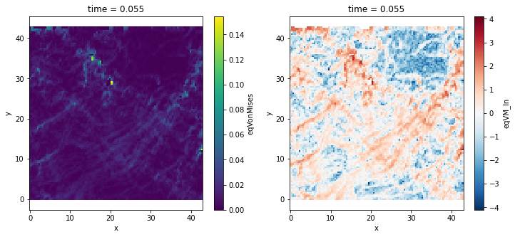
Compute the deformation equivalent
The deformation equivelent of \(\varepsilon\) is given by :
\(\varepsilon_{eq}=\sqrt{\frac{2}{3}\varepsilon_{ij}^d\varepsilon_{ij}^d}\)
with : \(\varepsilon^d=\varepsilon-\frac{1}{3}tr(\varepsilon)I\)
Definition from wikipedia
ds['eqVonMises']=ds.strain.sT.eqVonMises()
ds['eqVM_ln']=ds.strain.sT.eqVonMises(lognorm=True)
/home/chauvet/Documents/GitGricad/lib-python/xarray_symTensor2d/xarray_symTensor2d/xarray_symTensor2d.py:35: RuntimeWarning: divide by zero encountered in log
  deq[i,...]=np.log(deq[i,...]/med[i])
ds
<xarray.Dataset>
Dimensions:       (d: 2, sT: 6, time: 11, x: 108, y: 108)
Coordinates:
  * time          (time) float64 0.005 0.01 0.015 0.02 ... 0.04 0.045 0.05 0.055
  * x             (x) float64 0.0 0.4 0.8 1.2 1.6 ... 41.2 41.6 42.0 42.4 42.8
  * y             (y) float64 0.0 0.4 0.8 1.2 1.6 ... 41.2 41.6 42.0 42.4 42.8
Dimensions without coordinates: d, sT
Data variables:
    displacement  (time, y, x, d) float64 -0.01382 0.02172 ... 0.05585 0.2646
    strain        (time, y, x, sT) float64 -0.0003503 0.009625 nan ... nan nan
    eqVonMises    (time, y, x) float64 0.006643 0.00459 ... 0.0008373 0.00292
    eqVM_ln       (time, y, x) float64 0.3903 0.02058 -2.378 ... -1.885 -0.6359
Attributes:
    unit_time:      macro_strain
    step_size:      0.01
    unit_position:  millimeter
    window_size:    40
    path_dat:       /data/Manips/Columnar_Ice/CI23/DIC_Analysis/nm_analysis_0...
DIC_software: 7D- d: 2
- sT: 6
- time: 11
- x: 108
- y: 108
- time(time)float640.005 0.01 0.015 ... 0.05 0.055
array([0.005, 0.01 , 0.015, 0.02 , 0.025, 0.03 , 0.035, 0.04 , 0.045, 0.05 , 0.055]) - x(x)float640.0 0.4 0.8 1.2 ... 42.0 42.4 42.8
array([ 0. , 0.4, 0.8, 1.2, 1.6, 2. , 2.4, 2.8, 3.2, 3.6, 4. , 4.4, 4.8, 5.2, 5.6, 6. , 6.4, 6.8, 7.2, 7.6, 8. , 8.4, 8.8, 9.2, 9.6, 10. , 10.4, 10.8, 11.2, 11.6, 12. , 12.4, 12.8, 13.2, 13.6, 14. , 14.4, 14.8, 15.2, 15.6, 16. , 16.4, 16.8, 17.2, 17.6, 18. , 18.4, 18.8, 19.2, 19.6, 20. , 20.4, 20.8, 21.2, 21.6, 22. , 22.4, 22.8, 23.2, 23.6, 24. , 24.4, 24.8, 25.2, 25.6, 26. , 26.4, 26.8, 27.2, 27.6, 28. , 28.4, 28.8, 29.2, 29.6, 30. , 30.4, 30.8, 31.2, 31.6, 32. , 32.4, 32.8, 33.2, 33.6, 34. , 34.4, 34.8, 35.2, 35.6, 36. , 36.4, 36.8, 37.2, 37.6, 38. , 38.4, 38.8, 39.2, 39.6, 40. , 40.4, 40.8, 41.2, 41.6, 42. , 42.4, 42.8]) - y(y)float640.0 0.4 0.8 1.2 ... 42.0 42.4 42.8
array([ 0. ,  0.4,  0.8,  1.2,  1.6,  2. ,  2.4,  2.8,  3.2,  3.6,  4. ,  4.4,
        4.8,  5.2,  5.6,  6. ,  6.4,  6.8,  7.2,  7.6,  8. ,  8.4,  8.8,  9.2,
        9.6, 10. , 10.4, 10.8, 11.2, 11.6, 12. , 12.4, 12.8, 13.2, 13.6, 14. ,
       14.4, 14.8, 15.2, 15.6, 16. , 16.4, 16.8, 17.2, 17.6, 18. , 18.4, 18.8,
       19.2, 19.6, 20. , 20.4, 20.8, 21.2, 21.6, 22. , 22.4, 22.8, 23.2, 23.6,
       24. , 24.4, 24.8, 25.2, 25.6, 26. , 26.4, 26.8, 27.2, 27.6, 28. , 28.4,
       28.8, 29.2, 29.6, 30. , 30.4, 30.8, 31.2, 31.6, 32. , 32.4, 32.8, 33.2,
       33.6, 34. , 34.4, 34.8, 35.2, 35.6, 36. , 36.4, 36.8, 37.2, 37.6, 38. ,
       38.4, 38.8, 39.2, 39.6, 40. , 40.4, 40.8, 41.2, 41.6, 42. , 42.4, 42.8])
- displacement(time, y, x, d)float64-0.01382 0.02172 ... 0.05585 0.2646
array([[[[-0.0138176 , 0.02172363], [-0.01269367, 0.01667236], [-0.01334625, 0.01440186], ..., [ 0.10404297, 0.10395996], [ 0.10484131, 0.10501465], [ 0.10544434, 0.10472656]], [[-0.01522213, 0.01732422], [-0.01540913, 0.01399414], [-0.01498169, 0.01441284], ..., [ 0.10421265, 0.10360229], [ 0.10390991, 0.10512207], [ 0.1048877 , 0.10512207]], [[-0.01673748, 0.01780273], [-0.01681585, 0.01567993], [-0.01620945, 0.01436646], ..., ... ..., [ 0.05506348, 0.26319592], [ 0.0549292 , 0.26423786], [ 0.05506836, 0.26406746]], [[ nan, nan], [ 0.0068755 , 0.26888802], [ 0.00852865, 0.27011887], ..., [ 0.05532104, 0.26495453], [ 0.05540283, 0.2654261 ], [ 0.0554126 , 0.26554352]], [[ nan, nan], [-0.01929932, 0.30371521], [-0.00242554, 0.3003447 ], ..., [ 0.05619141, 0.26459679], [ 0.05521484, 0.26542751], [ 0.05584961, 0.26460365]]]]) - strain(time, y, x, sT)float64-0.0003503 0.009625 nan ... nan nan
array([[[[-3.50349874e-04, 9.62528773e-03, nan, -1.80607068e-03, nan, nan], [ 1.87318481e-03, 6.62416639e-03, nan, -7.78798712e-05, nan, nan], [-5.29296813e-04, -1.24854778e-04, nan, 2.18693574e-04, nan, nan], ..., [-7.77722598e-05, 6.72160764e-04, nan, 1.28303189e-03, nan, nan], [ 2.08509131e-03, -1.70079205e-04, nan, 1.11463387e-03, nan, nan], [ 9.89774591e-04, -9.75468662e-04, nan, 2.54816969e-05, nan, nan]], [[-2.83982634e-04, 3.67443566e-03, nan, -1.96263939e-03, nan, nan], [ 1.30781333e-03, 1.09543174e-03, nan, -5.09590784e-04, nan, nan], [-5.84078138e-04, -4.11169640e-06, nan, 1.57794810e-03, nan, nan], ... [ 1.15511520e-03, -1.54172420e-03, nan, -6.96854375e-04, nan, nan], [-3.48088914e-04, -2.59150728e-03, nan, -6.05857756e-04, nan, nan], [ 1.08583318e-03, 8.78957042e-04, nan, 7.23363657e-04, nan, nan]], [[ nan, nan, nan, nan, nan, nan], [ 4.31097373e-02, -7.81000406e-02, nan, 3.00260577e-02, nan, nan], [-5.50938203e-05, -6.76996037e-02, nan, 3.52105387e-02, nan, nan], ..., [ 8.44421913e-04, -2.16673798e-04, nan, 1.30847562e-04, nan, nan], [ 4.10129986e-04, -1.11063570e-03, nan, -2.96394021e-04, nan, nan], [ 2.40789144e-03, 3.42831877e-03, nan, 9.04984598e-04, nan, nan]]]]) - eqVonMises(time, y, x)float640.006643 0.00459 ... 0.00292
array([[[0.00664305, 0.00458987, 0.00041708, ..., 0.00129103, 0.00174628, 0.00092676], [0.00307579, 0.00123463, 0.00153782, ..., 0.00153045, 0.00137174, 0.00158594], [0.00239769, 0.00238624, 0.00386586, ..., 0.0024106 , 0.00083552, 0.00159646], ..., [0.01420932, 0.01073608, 0.00990502, ..., 0.00602953, 0.00365314, 0.00194513], [0.02188799, 0.01488689, 0.01270582, ..., 0.00209061, 0.00473817, 0.00219811], [0. , 0.0174847 , 0.01994319, ..., 0.00228945, 0.00439212, 0.00630271]], [[0.00804353, 0.00849724, 0.00740109, ..., 0.00136193, 0.00209083, 0.00335859], [0.00600652, 0.00610367, 0.00436017, ..., 0.00272155, 0.00250041, 0.00169492], [0.00604149, 0.00676466, 0.00466716, ..., 0.00255971, 0.00097829, 0.00526355], ... [0.02095929, 0.03673353, 0.04022176, ..., 0.01034013, 0.00568373, 0.00398989], [0.03709792, 0.05301696, 0.05738432, ..., 0.01031634, 0.00224696, 0.00155169], [0.05021062, 0.05265029, 0.0657613 , ..., 0.00883416, 0.00358037, 0.00336707]], [[0.00830681, 0.00724994, 0.0075008 , ..., 0.00254831, 0.0104371 , 0.01869162], [0.00619591, 0.00424121, 0.00425377, ..., 0.00736972, 0.01389624, 0.01794475], [0.00397934, 0.00181282, 0.00087594, ..., 0.00586268, 0.0116237 , 0.01862643], ..., [0.0189354 , 0.0380885 , 0.05805568, ..., 0.00598112, 0.00812369, 0.00802149], [0. , 0.05434984, 0.05305789, ..., 0.00144259, 0.00183439, 0.00115434], [0. , 0.06586584, 0.05602699, ..., 0.00059413, 0.0008373 , 0.00292037]]]) - eqVM_ln(time, y, x)float640.3903 0.02058 ... -1.885 -0.6359
array([[[ 0.39030386,  0.0205846 , -2.37774781, ..., -1.24782883,
         -0.94578001, -1.57932708],
        [-0.37970662, -1.29249398, -1.07290106, ..., -1.07770612,
         -1.18718579, -1.04208901],
        [-0.62875977, -0.63354906, -0.15108301, ..., -0.62338955,
         -1.68296641, -1.03547954],
        ...,
        [ 1.15063083,  0.87034346,  0.78977457, ...,  0.29340132,
         -0.20767859, -0.83793867],
        [ 1.58267119,  1.19721363,  1.03879288, ..., -0.76581349,
          0.05238358, -0.71566763],
        [       -inf,  1.35805899,  1.48962057, ..., -0.67495634,
         -0.023454  ,  0.33771335]],

       [[ 0.36523186,  0.42010566,  0.28199115, ..., -1.41073597,
         -0.98207548, -0.50811369],
        [ 0.07320922,  0.08925373, -0.24712505, ..., -0.71843333,
         -0.80318166, -1.19199958],
        [ 0.07901393,  0.19207601, -0.17908532, ..., -0.77974235,
         -1.74158883, -0.05883088],
...
        [ 1.37511729,  1.93622536,  2.02694365, ...,  0.66856815,
          0.0701435 , -0.2836999 ],
        [ 1.94609642,  2.3031474 ,  2.38230653, ...,  0.66626457,
         -0.85788435, -1.22812131],
        [ 2.24876206,  2.29620722,  2.51856689, ...,  0.51116152,
         -0.39199857, -0.45342085]],

       [[ 0.40948814,  0.27340638,  0.30742211, ..., -0.77215872,
          0.63777917,  1.2204879 ],
        [ 0.11630245, -0.26273845, -0.25978261, ...,  0.28979284,
          0.92403107,  1.17971043],
        [-0.32647108, -1.11270324, -1.8400473 , ...,  0.06101956,
          0.74545919,  1.21699427],
        ...,
        [ 1.23344603,  1.932325  ,  2.35381535, ...,  0.08102087,
          0.38719682,  0.37453669],
        [       -inf,  2.28785436,  2.26379623, ..., -1.34114521,
         -1.10087639, -1.56406148],
        [       -inf,  2.48003262,  2.31824629, ..., -2.2282384 ,
         -1.88515801, -0.63587584]]])
- unit_time :
- macro_strain
- step_size :
- 0.01
- unit_position :
- millimeter
- window_size :
- 40
- path_dat :
- /data/Manips/Columnar_Ice/CI23/DIC_Analysis/nm_analysis_0.5pc/n40/
- DIC_software :
- 7D
plt.figure(figsize=(12,5))
plt.subplot(121)
ds.eqVonMises[ts].plot()
plt.axis('equal')
plt.subplot(122)
ds.eqVM_ln[ts].plot()
plt.axis('equal')
(-0.2, 43.0, -0.2, 43.0)
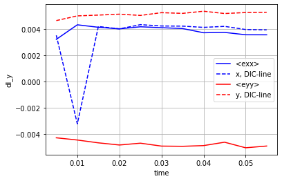
Compute the macroscopic strain
Compute the average of the strain tensor
ds['mean_eyy']=ds.strain.sT.mean('tyy')
ds['mean_exx']=ds.strain.sT.mean('txx')
Compute the DIC_line
The DIC_line is defined in 1, section 2.2.3.1
ds['dl_x']=ds.dic.DIC_line('x')
ds['dl_y']=ds.dic.DIC_line('y')
plt.figure()
ds.mean_exx.plot.line('b-',label='<exx>')
ds.dl_x.plot.line('b--',label='x, DIC-line')
ds.mean_eyy.plot.line('r-',label='<eyy>')
ds.dl_y.plot.line('r--',label='y, DIC-line')
plt.grid()
plt.legend()
<matplotlib.legend.Legend at 0x7fa927990100>
ds
<xarray.Dataset>
Dimensions:       (d: 2, sT: 6, time: 11, x: 108, y: 108)
Coordinates:
  * time          (time) float64 0.005 0.01 0.015 0.02 ... 0.04 0.045 0.05 0.055
  * x             (x) float64 0.0 0.4 0.8 1.2 1.6 ... 41.2 41.6 42.0 42.4 42.8
  * y             (y) float64 0.0 0.4 0.8 1.2 1.6 ... 41.2 41.6 42.0 42.4 42.8
Dimensions without coordinates: d, sT
Data variables:
    displacement  (time, y, x, d) float64 -0.01382 0.02172 ... 0.05585 0.2646
    strain        (time, y, x, sT) float64 -0.0003503 0.009625 nan ... nan nan
    eqVonMises    (time, y, x) float64 0.006643 0.00459 ... 0.0008373 0.00292
    eqVM_ln       (time, y, x) float64 0.3903 0.02058 -2.378 ... -1.885 -0.6359
    mean_eyy      (time) float64 -0.004295 -0.004464 ... -0.005055 -0.004922
    mean_exx      (time) float64 0.003198 0.004306 ... 0.003548 0.003545
    dl_x          (time) float64 0.003503 -0.003233 ... 0.003946 0.00392
    dl_y          (time) float64 0.004627 0.004986 ... 0.005239 0.005256
Attributes:
    unit_time:      macro_strain
    step_size:      0.01
    unit_position:  millimeter
    window_size:    40
    path_dat:       /data/Manips/Columnar_Ice/CI23/DIC_Analysis/nm_analysis_0...
DIC_software: 7D- d: 2
- sT: 6
- time: 11
- x: 108
- y: 108
- time(time)float640.005 0.01 0.015 ... 0.05 0.055
array([0.005, 0.01 , 0.015, 0.02 , 0.025, 0.03 , 0.035, 0.04 , 0.045, 0.05 , 0.055]) - x(x)float640.0 0.4 0.8 1.2 ... 42.0 42.4 42.8
array([ 0. , 0.4, 0.8, 1.2, 1.6, 2. , 2.4, 2.8, 3.2, 3.6, 4. , 4.4, 4.8, 5.2, 5.6, 6. , 6.4, 6.8, 7.2, 7.6, 8. , 8.4, 8.8, 9.2, 9.6, 10. , 10.4, 10.8, 11.2, 11.6, 12. , 12.4, 12.8, 13.2, 13.6, 14. , 14.4, 14.8, 15.2, 15.6, 16. , 16.4, 16.8, 17.2, 17.6, 18. , 18.4, 18.8, 19.2, 19.6, 20. , 20.4, 20.8, 21.2, 21.6, 22. , 22.4, 22.8, 23.2, 23.6, 24. , 24.4, 24.8, 25.2, 25.6, 26. , 26.4, 26.8, 27.2, 27.6, 28. , 28.4, 28.8, 29.2, 29.6, 30. , 30.4, 30.8, 31.2, 31.6, 32. , 32.4, 32.8, 33.2, 33.6, 34. , 34.4, 34.8, 35.2, 35.6, 36. , 36.4, 36.8, 37.2, 37.6, 38. , 38.4, 38.8, 39.2, 39.6, 40. , 40.4, 40.8, 41.2, 41.6, 42. , 42.4, 42.8]) - y(y)float640.0 0.4 0.8 1.2 ... 42.0 42.4 42.8
array([ 0. ,  0.4,  0.8,  1.2,  1.6,  2. ,  2.4,  2.8,  3.2,  3.6,  4. ,  4.4,
        4.8,  5.2,  5.6,  6. ,  6.4,  6.8,  7.2,  7.6,  8. ,  8.4,  8.8,  9.2,
        9.6, 10. , 10.4, 10.8, 11.2, 11.6, 12. , 12.4, 12.8, 13.2, 13.6, 14. ,
       14.4, 14.8, 15.2, 15.6, 16. , 16.4, 16.8, 17.2, 17.6, 18. , 18.4, 18.8,
       19.2, 19.6, 20. , 20.4, 20.8, 21.2, 21.6, 22. , 22.4, 22.8, 23.2, 23.6,
       24. , 24.4, 24.8, 25.2, 25.6, 26. , 26.4, 26.8, 27.2, 27.6, 28. , 28.4,
       28.8, 29.2, 29.6, 30. , 30.4, 30.8, 31.2, 31.6, 32. , 32.4, 32.8, 33.2,
       33.6, 34. , 34.4, 34.8, 35.2, 35.6, 36. , 36.4, 36.8, 37.2, 37.6, 38. ,
       38.4, 38.8, 39.2, 39.6, 40. , 40.4, 40.8, 41.2, 41.6, 42. , 42.4, 42.8])
- displacement(time, y, x, d)float64-0.01382 0.02172 ... 0.05585 0.2646
array([[[[-0.0138176 , 0.02172363], [-0.01269367, 0.01667236], [-0.01334625, 0.01440186], ..., [ 0.10404297, 0.10395996], [ 0.10484131, 0.10501465], [ 0.10544434, 0.10472656]], [[-0.01522213, 0.01732422], [-0.01540913, 0.01399414], [-0.01498169, 0.01441284], ..., [ 0.10421265, 0.10360229], [ 0.10390991, 0.10512207], [ 0.1048877 , 0.10512207]], [[-0.01673748, 0.01780273], [-0.01681585, 0.01567993], [-0.01620945, 0.01436646], ..., ... ..., [ 0.05506348, 0.26319592], [ 0.0549292 , 0.26423786], [ 0.05506836, 0.26406746]], [[ nan, nan], [ 0.0068755 , 0.26888802], [ 0.00852865, 0.27011887], ..., [ 0.05532104, 0.26495453], [ 0.05540283, 0.2654261 ], [ 0.0554126 , 0.26554352]], [[ nan, nan], [-0.01929932, 0.30371521], [-0.00242554, 0.3003447 ], ..., [ 0.05619141, 0.26459679], [ 0.05521484, 0.26542751], [ 0.05584961, 0.26460365]]]]) - strain(time, y, x, sT)float64-0.0003503 0.009625 nan ... nan nan
array([[[[-3.50349874e-04, 9.62528773e-03, nan, -1.80607068e-03, nan, nan], [ 1.87318481e-03, 6.62416639e-03, nan, -7.78798712e-05, nan, nan], [-5.29296813e-04, -1.24854778e-04, nan, 2.18693574e-04, nan, nan], ..., [-7.77722598e-05, 6.72160764e-04, nan, 1.28303189e-03, nan, nan], [ 2.08509131e-03, -1.70079205e-04, nan, 1.11463387e-03, nan, nan], [ 9.89774591e-04, -9.75468662e-04, nan, 2.54816969e-05, nan, nan]], [[-2.83982634e-04, 3.67443566e-03, nan, -1.96263939e-03, nan, nan], [ 1.30781333e-03, 1.09543174e-03, nan, -5.09590784e-04, nan, nan], [-5.84078138e-04, -4.11169640e-06, nan, 1.57794810e-03, nan, nan], ... [ 1.15511520e-03, -1.54172420e-03, nan, -6.96854375e-04, nan, nan], [-3.48088914e-04, -2.59150728e-03, nan, -6.05857756e-04, nan, nan], [ 1.08583318e-03, 8.78957042e-04, nan, 7.23363657e-04, nan, nan]], [[ nan, nan, nan, nan, nan, nan], [ 4.31097373e-02, -7.81000406e-02, nan, 3.00260577e-02, nan, nan], [-5.50938203e-05, -6.76996037e-02, nan, 3.52105387e-02, nan, nan], ..., [ 8.44421913e-04, -2.16673798e-04, nan, 1.30847562e-04, nan, nan], [ 4.10129986e-04, -1.11063570e-03, nan, -2.96394021e-04, nan, nan], [ 2.40789144e-03, 3.42831877e-03, nan, 9.04984598e-04, nan, nan]]]]) - eqVonMises(time, y, x)float640.006643 0.00459 ... 0.00292
array([[[0.00664305, 0.00458987, 0.00041708, ..., 0.00129103, 0.00174628, 0.00092676], [0.00307579, 0.00123463, 0.00153782, ..., 0.00153045, 0.00137174, 0.00158594], [0.00239769, 0.00238624, 0.00386586, ..., 0.0024106 , 0.00083552, 0.00159646], ..., [0.01420932, 0.01073608, 0.00990502, ..., 0.00602953, 0.00365314, 0.00194513], [0.02188799, 0.01488689, 0.01270582, ..., 0.00209061, 0.00473817, 0.00219811], [0. , 0.0174847 , 0.01994319, ..., 0.00228945, 0.00439212, 0.00630271]], [[0.00804353, 0.00849724, 0.00740109, ..., 0.00136193, 0.00209083, 0.00335859], [0.00600652, 0.00610367, 0.00436017, ..., 0.00272155, 0.00250041, 0.00169492], [0.00604149, 0.00676466, 0.00466716, ..., 0.00255971, 0.00097829, 0.00526355], ... [0.02095929, 0.03673353, 0.04022176, ..., 0.01034013, 0.00568373, 0.00398989], [0.03709792, 0.05301696, 0.05738432, ..., 0.01031634, 0.00224696, 0.00155169], [0.05021062, 0.05265029, 0.0657613 , ..., 0.00883416, 0.00358037, 0.00336707]], [[0.00830681, 0.00724994, 0.0075008 , ..., 0.00254831, 0.0104371 , 0.01869162], [0.00619591, 0.00424121, 0.00425377, ..., 0.00736972, 0.01389624, 0.01794475], [0.00397934, 0.00181282, 0.00087594, ..., 0.00586268, 0.0116237 , 0.01862643], ..., [0.0189354 , 0.0380885 , 0.05805568, ..., 0.00598112, 0.00812369, 0.00802149], [0. , 0.05434984, 0.05305789, ..., 0.00144259, 0.00183439, 0.00115434], [0. , 0.06586584, 0.05602699, ..., 0.00059413, 0.0008373 , 0.00292037]]]) - eqVM_ln(time, y, x)float640.3903 0.02058 ... -1.885 -0.6359
array([[[ 0.39030386, 0.0205846 , -2.37774781, ..., -1.24782883, -0.94578001, -1.57932708], [-0.37970662, -1.29249398, -1.07290106, ..., -1.07770612, -1.18718579, -1.04208901], [-0.62875977, -0.63354906, -0.15108301, ..., -0.62338955, -1.68296641, -1.03547954], ..., [ 1.15063083, 0.87034346, 0.78977457, ..., 0.29340132, -0.20767859, -0.83793867], [ 1.58267119, 1.19721363, 1.03879288, ..., -0.76581349, 0.05238358, -0.71566763], [ -inf, 1.35805899, 1.48962057, ..., -0.67495634, -0.023454 , 0.33771335]], [[ 0.36523186, 0.42010566, 0.28199115, ..., -1.41073597, -0.98207548, -0.50811369], [ 0.07320922, 0.08925373, -0.24712505, ..., -0.71843333, -0.80318166, -1.19199958], [ 0.07901393, 0.19207601, -0.17908532, ..., -0.77974235, -1.74158883, -0.05883088], ... [ 1.37511729, 1.93622536, 2.02694365, ..., 0.66856815, 0.0701435 , -0.2836999 ], [ 1.94609642, 2.3031474 , 2.38230653, ..., 0.66626457, -0.85788435, -1.22812131], [ 2.24876206, 2.29620722, 2.51856689, ..., 0.51116152, -0.39199857, -0.45342085]], [[ 0.40948814, 0.27340638, 0.30742211, ..., -0.77215872, 0.63777917, 1.2204879 ], [ 0.11630245, -0.26273845, -0.25978261, ..., 0.28979284, 0.92403107, 1.17971043], [-0.32647108, -1.11270324, -1.8400473 , ..., 0.06101956, 0.74545919, 1.21699427], ..., [ 1.23344603, 1.932325 , 2.35381535, ..., 0.08102087, 0.38719682, 0.37453669], [ -inf, 2.28785436, 2.26379623, ..., -1.34114521, -1.10087639, -1.56406148], [ -inf, 2.48003262, 2.31824629, ..., -2.2282384 , -1.88515801, -0.63587584]]]) - mean_eyy(time)float64-0.004295 -0.004464 ... -0.004922
array([-0.00429511, -0.00446444, -0.00467952, -0.00484299, -0.00470528, -0.00492744, -0.00494307, -0.0048891 , -0.0046311 , -0.00505546, -0.00492185]) - mean_exx(time)float640.003198 0.004306 ... 0.003545
array([0.00319824, 0.00430589, 0.0041179 , 0.00399834, 0.00415583, 0.00408559, 0.00402246, 0.00370215, 0.0037277 , 0.00354776, 0.00354507]) - dl_x(time)float640.003503 -0.003233 ... 0.00392
array([ 0.00350296, -0.0032332 , 0.00417895, 0.00399622, 0.00431765, 0.00421546, 0.00420573, 0.00411067, 0.00418713, 0.00394596, 0.00391961]) - dl_y(time)float640.004627 0.004986 ... 0.005256
array([0.00462724, 0.00498554, 0.00504535, 0.0051154 , 0.00502004,
       0.00523006, 0.00517625, 0.00533973, 0.00516498, 0.00523933,
       0.0052559 ])
- unit_time :
- macro_strain
- step_size :
- 0.01
- unit_position :
- millimeter
- window_size :
- 40
- path_dat :
- /data/Manips/Columnar_Ice/CI23/DIC_Analysis/nm_analysis_0.5pc/n40/
- DIC_software :
- 7D
Extract image number each XX marcro strain
Macro strain wanted between 2 images.
strain_step=-0.005
offset and nb of image at each time
im_nb_offset=0
im_nb_time=1
Extract the number of the image
name_im=ds.dic.find_pic(strain_step=strain_step,a_im=im_nb_time,b_im=im_nb_offset,axis='y')
print(name_im)
[]
Performed Auto Correlation analysis
import xarray_function.image as xfi
ds_auto0=xfi.auto_correlation(ds.eqVonMises[0,:,:],pad=1)
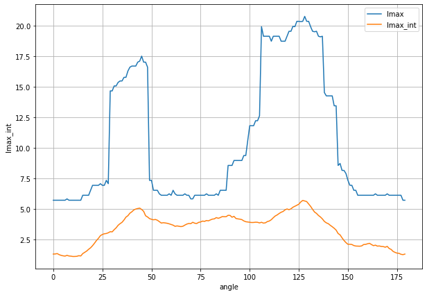
Plot correlation length
Plot the correlation length in function of the angle.
Angle = 90° correspond to +y direction
Angle = 0° correspond to +x direction
Angle = +180° correspond to -x direction
plt.figure(figsize=(10,7))
ds_auto0.lmax.plot(label='lmax')
ds_auto0.lmax_int.plot(label='lmax_int')
plt.grid()
plt.legend()
<matplotlib.legend.Legend at 0x7fa92a73ee50>
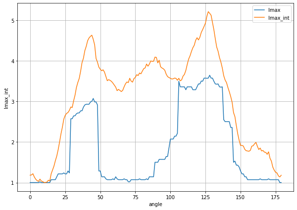
plt.figure(figsize=(10,7))
(ds_auto0.lmax/ds_auto0.lmax.min()).plot(label='lmax')
(ds_auto0.lmax_int/ds_auto0.lmax_int.min()).plot(label='lmax_int')
plt.grid()
plt.legend()
<matplotlib.legend.Legend at 0x7fa92a6864f0>
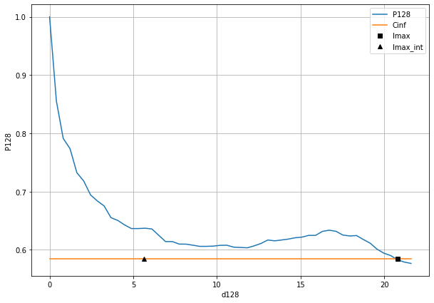
Plot correlation profil along one direction
Correlation profil are compute at every integer angle between \([0,179]\). They are store in ds_auto0 and you can plot those.
You can find the angle for which the corrlation length is maximal
idm=np.where(ds_auto0.lmax==np.max(ds_auto0.lmax))
And plot the profil
plt.figure(figsize=(10,7))
ds_auto0['P'+str(idm[0][0])].plot(label='P'+str(idm[0][0]))
plt.plot([0,ds_auto0['d'+str(idm[0][0])][-1]],[ds_auto0.Cinf,ds_auto0.Cinf],label='Cinf')
plt.plot(ds_auto0.lmax[idm[0][0]],ds_auto0.Cinf,'sk',label='lmax')
plt.plot(ds_auto0.lmax_int[idm[0][0]],ds_auto0.Cinf,'^k',label='lmax_int')
plt.grid()
plt.legend()
<matplotlib.legend.Legend at 0x7fa9279056a0>