Perform segmentation#
Warning
This notebook shows how to use a function that is poorly written and not optimized. The results from this function are also to be taken carefully.
This notebook show how to segment your data to find grain boundaries and create the so-called microstructure data.
import xarrayaita.loadData_aita as lda #here are some function to build xarrayaita structure
import xarrayaita.aita as xa
import xarrayuvecs.uvecs as xu
import xarrayuvecs.lut2d as lut2d

import matplotlib.pyplot as plt
import matplotlib.cm as cm
import numpy as np

import datetime
from skimage import morphology
from tqdm.notebook import tqdm
import scipy

%matplotlib widget
Load your data#
# path to data
path_data='orientation_test.dat'
data=lda.aita5col(path_data)
data
<xarray.Dataset>
Dimensions:      (y: 2500, x: 1000, uvecs: 2)
Coordinates:
  * x            (x) float64 0.0 0.02 0.04 0.06 0.08 ... 19.92 19.94 19.96 19.98
  * y            (y) float64 49.98 49.96 49.94 49.92 49.9 ... 0.06 0.04 0.02 0.0
Dimensions without coordinates: uvecs
Data variables:
    orientation  (y, x, uvecs) float64 2.395 0.6451 5.377 ... 0.6098 0.6473
    quality      (y, x) int64 0 90 92 93 92 92 94 94 ... 96 96 96 96 96 97 97 96
    micro        (y, x) float64 0.0 0.0 0.0 0.0 0.0 0.0 ... 0.0 0.0 0.0 0.0 0.0
    grainId      (y, x) int64 1 1 1 1 1 1 1 1 1 1 1 1 ... 1 1 1 1 1 1 1 1 1 1 1
Attributes:
    date:       Thursday, 19 Nov 2015, 11:24 am
    unit:       millimeters
    step_size:  0.02
path_dat: orientation_test.datSegment the data#
plt.figure(figsize=(5,10))
out=data.aita.interactive_segmentation()
The new xarray.DataSet.aita#
out.ds
<xarray.Dataset>
Dimensions:      (y: 2500, x: 1000, uvecs: 2)
Coordinates:
  * y            (y) float64 49.98 49.96 49.94 49.92 49.9 ... 0.06 0.04 0.02 0.0
  * x            (x) float64 0.0 0.02 0.04 0.06 0.08 ... 19.92 19.94 19.96 19.98
Dimensions without coordinates: uvecs
Data variables:
    orientation  (y, x, uvecs) float64 2.395 0.6451 5.377 ... 0.6098 0.6473
    quality      (y, x) int64 0 90 92 93 92 92 94 94 ... 96 96 96 96 96 97 97 96
    micro        (y, x) bool False False False False ... False False False False
    grainId      (y, x) int32 1 1 1 1 1 1 1 1 ... 962 962 962 962 962 962 962
Attributes:
    date:       Thursday, 19 Nov 2015, 11:24 am
    unit:       millimeters
    step_size:  0.02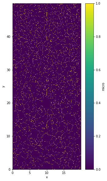
path_dat: orientation_test.datPlot the microstructure#
%matplotlib inline
plt.figure(figsize=(5,10))
out.ds.micro.plot()
<matplotlib.collections.QuadMesh at 0x7f3f36571790>
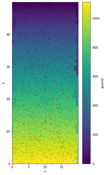
Plot grainId#
plt.figure(figsize=(5,10))
out.ds.grainId.plot()
<matplotlib.collections.QuadMesh at 0x7f3f364c5880>
Parameters of the segmentation#
If you want to re-do the segmentation with the same value they can be found here :
print('Use scharr:',out.use_scharr)
print('Value scharr:',out.val_scharr)
print('Use canny:',out.use_canny)
print('Value canny:',out.val_canny)
print('Images canny:',out.img_canny)
print('Use quality:',out.use_quality)
print('Value quality:',out.val_quality)
print('Include border:',out.include_border)
Use scharr: True
Value scharr: 1.5
Use canny: True
Value canny: 1.5
Images canny: semi color wheel
Use quality: False
Value quality: 60.0
Include border: False
Export the segmentation#
Manual corrections are often necessary after this step.
plt.imsave('micro auto.bmp', np.array(out.ds.micro), cmap=cm.gray)